Model-Based Reinforcement Learning¶

Model-Based Reinforcement Learning (Model-Based RL) is an important branch of reinforcement learning. The agent learns a dynamics model by interacting with the environment and then uses the model to generate data to optimize policy or use the model for planning. The Model-Based RL method first learns a dynamics model from the data obtained by interacting with the environment and then uses the dynamics model to generate a large number of simulated samples. In this way, the number of interactions with the real environment will be reduced, or in other words, the sample efficiency can be greatly improved.

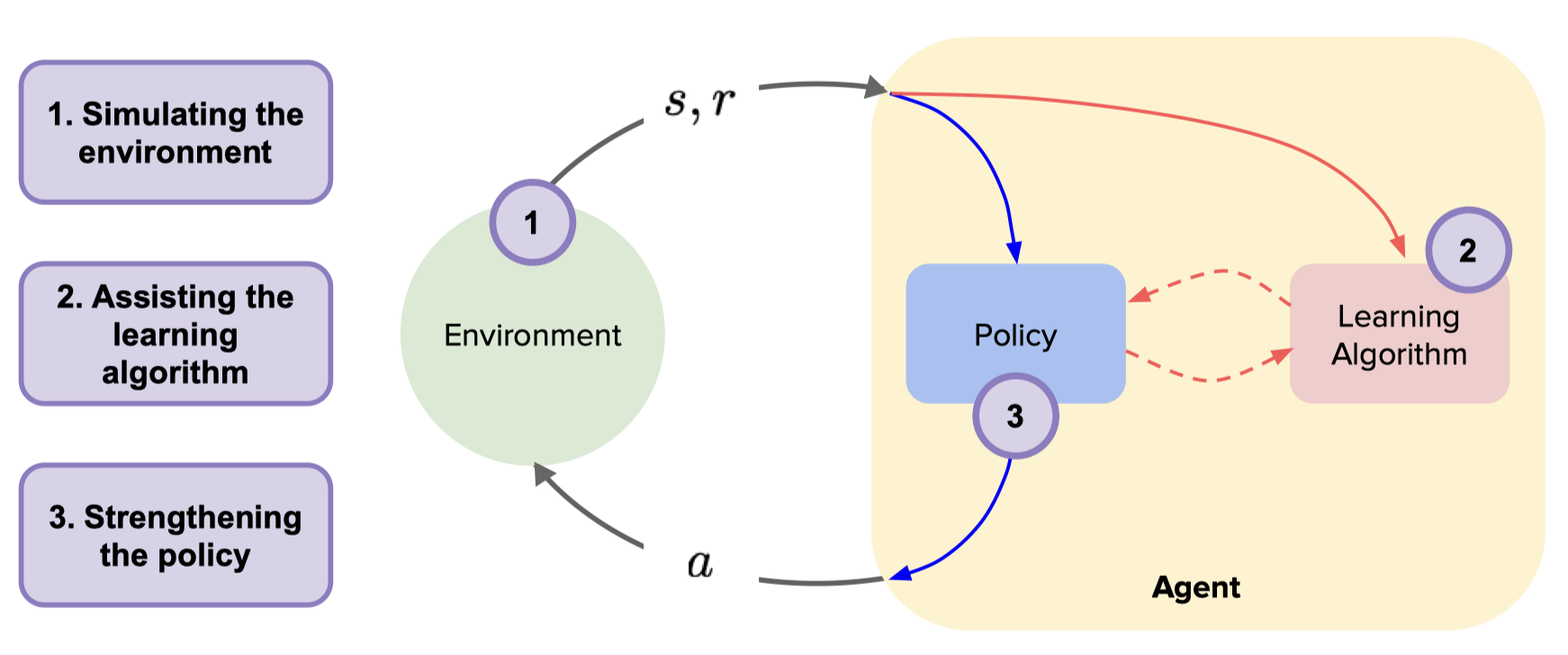
The environment model can generally be abstracted mathematically into a state transition function and a reward function. In the ideal case, the agent does not need to interact with the real environment anymore after learning the dynamics model. The agent can now query the dynamics model to produce simulated samples, by which the cumulative discount reward can be maximized to obtain the optimal policy.

Problem Definition and Research Motivation¶

In general, the problems of Model-Based RL research can be divided into two categories: how to learn an accurate dynamics model, and how to use the dynamics model for policy optimization.

How to build an accurate environment model?

Model learning mainly emphasizes the process of building an environment model by the Model-Based RL algorithm. For example,

World Model 3 proposes an environment model based on unsupervised learning and uses this model to transfer tasks from simulation to reality.

I2A 4 proposes an imagination-augmented-based model structure, based on which the future trajectory is predicted, and the trajectory information is encoded to assist policy learning.

But Model-Based RL also has several problems in the model learning part, for example,

There will be errors in the dynamics model, and with the iterative interaction between the agent and the dynamics model, the error induced by the model will compound over time, making it difficult for the algorithm to converge to the optimal solution.

The environment model lacks generality, and every time a problem is changed, the model must be re-modeled.

How to use the environment model for policy optimization?

Model utilization mainly emphasizes that Model-Based RL algorithms use dynamics models to assist policy learning, such as model-based planning or model-based policy learning.

Both ExIt 5 and AlphaZero 6 are based on expert iteration and Monte Carlo tree search methods to learn strategies.

POPLIN 7 does online planning based on the environment model, and proposes optimization ideas for action space and parameter space respectively.

M2AC 8 proposes a mask mechanism based on model uncertainty, which enhances policy improvement.

Research Direction¶

The papers of Model-Based RL in recent years have been sorted out and summarized in awesome-model-based-RL 1. One of the most classic Model-Based RL algorithms is Dyna-style reinforcement learning, which is a type of algorithm that combines Model-Based RL and Model-Free RL. In addition to the classic Dyna-style reinforcement learning, there are roughly the following categories of model-based reinforcement learning:

Model-Based Planning Algorithms
Model-Based Value Extension Reinforcement Learning
Policy Optimization Combined with Model Gradient Backhaul

Model-Based Planning Algorithms¶

After learning the dynamics model of the environment, the model can be directly used for planning. At this time, reinforcement learning can be transformed into an optimal control problem: the optimal strategy can be obtained through the planning algorithm, and the planning algorithm can also be used to generate better samples to assist learning. The most common of this type of algorithms is the Cross Entropy Method (CEM). Its idea is to assume that the action sequence obeys a certain prior distribution, sample actions to obtain trajectories, and select a good trajectory to update the prior distribution a posteriori.

The model-based planning algorithm is roughly divided into three steps in each iteration:

In the first step, after performing an action, predict the next state according to the environment dynamics model.
The second step is to use algorithms such as CEM to solve the action sequence.
In the third step, perform the first action solved in the second step, and so on.

Typical algorithms of this type are RS 9, PETS 10, POPLIN 7. However, when solving high-dimensional control tasks, the difficulty of planning and the required computation will increase significantly, and the planning effect will become worse, so it is suitable for simple models with low action dimensions.

Model-Based Value Extension Reinforcement Learning¶

The model-based planning algorithm inputs a state every time, and needs to plan again to obtain the output action, while a trained strategy directly maps the state to an action, and the trained strategy is faster than the planning algorithm in practical applications. In the combined mode of Model-Based and Model-Free, the model error will reduce the performance of the entire algorithm. MVE 11 estimates the value function by using the environment model rollout to generate a fixed number of H-step trajectories for Model-Based Value Expansion. Therefore, the estimation of the Q value integrates the short-term prediction based on the environmental dynamics model and the long-term prediction based on the target Q value network. The number of steps H limits the accumulation of compound errors and improves the accuracy of the Q value.

STEVE 12 pointed out that MVE needs to rely on the adjustment of the number of steps H of the rollout, that is, in a complex environment, if the number of steps in the model is too large, a large error will be introduced, while in a simple environment, if the number of steps is too small, it will reduce the estimation accuracy of the Q value. Therefore, STEVE deploys different specific steps in different environments, calculates the uncertainty of each step, dynamically adjusts and integrates the weight of the Q value between different steps, so that the Q value prediction under each environmental task is more accurate.

Policy Optimization Combined with Model Gradient Backhaul¶

In addition to using the virtual expansion of the model to generate data, if the model is a neural network or other differentiable functions, the differentiable characteristics of the model can also be used to directly assist the learning of the strategy. This method further utilizes the model.

SVG 13 uses real samples to fit the model, and optimizes the value function by using the differentiability of the model, that is, using the chain rule and the differentiability of the model to directly derive the value function, and use the gradient ascent method to optimize the value function and learn the strategy. Only real samples are used in the optimization process, and the model is not used to generate virtual data. The advantage of this is that it can alleviate the impact of inaccurate models, but at the same time, because the model is not used to generate dummy data, the sample efficiency has not been greatly improved.

In addition to using the gradient of the model, MAAC 14 uses the Q-value function of H-step bootstrapping as the objective function of reinforcement learning. At the same time, the data in the replay buffer includes both the data interacting with the real environment and the data of the virtual expansion of the model. The hyperparameter H can make the objective function trade-off between the accuracy of the model and the accuracy of the Q-value function. Calculating gradients with backpropagation using model differentiability may encounter a class of problems that exist in deep learning, gradient vanishing and gradient exploding. The Terminal Q-Function is used in MAAC to alleviate this problem. SVG 13 and Dreamer 15 are implemented using gradient clipping tricks. In addition, using the differentiability of the model may also fall into the problem of local optima during gradient optimization. 2

Future Study¶

Model-based reinforcement learning has high sample efficiency, but the training process of environmental models is often time-intensive, so “how to improve the learning efficiency of the model” is very necessary.
In addition, due to the lack of generality of the environment model, it is often necessary to re-model every time a problem is changed. In order to solve the problem of model generalization between different tasks, “how to introduce the ideas and techniques of transfer learning and meta-learning into model-based reinforcement learning” is also a very important research question.
Model-based reinforcement learning modeling and decision-making on high-dimensional image observations, as well as model-based reinforcement learning combined with Offline RL, will be sufficient conditions for future reinforcement learning to lead to Sim2Real.

References¶

1: Repo: awesome-model-based-RL. https://github.com/opendilab/awesome-model-based-RL
2: Sun S, Lan X, Zhang H, Zheng N. Model-Based Reinforcement Learning in Robotics: A Survey[J]. Pattern Recognition and Artificial Intelligence, 2022, 35(01): 1-16. DOI: 10.16451/j.cnki.issn1003-6059.202201001.
3: Ha D, Schmidhuber J. World models[J]. arXiv preprint arXiv:1803.10122, 2018.
4: Racanière S, Weber T, Reichert D, et al. Imagination-augmented agents for deep reinforcement learning[J]. Advances in neural information processing systems, 2017, 30.
5: Anthony T, Tian Z, Barber D. Thinking fast and slow with deep learning and tree search[J]. Advances in Neural Information Processing Systems, 2017, 30.
6: Silver D, Hubert T, Schrittwieser J, et al. Mastering chess and shogi by self-play with a general reinforcement learning algorithm[J]. arXiv preprint arXiv:1712.01815, 2017.
7(1,2): Wang T, Ba J. Exploring Model-based Planning with Policy Networks[C]//International Conference on Learning Representations. 2019.
8: Pan F, He J, Tu D, et al. Trust the model when it is confident: Masked model-based actor-critic[J]. Advances in neural information processing systems, 2020, 33: 10537-10546.
9: Richards A G. Robust constrained model predictive control[D]. Massachusetts Institute of Technology, 2005.
10: Chua K, Calandra R, McAllister R, et al. Deep reinforcement learning in a handful of trials using probabilistic dynamics models[J]. Advances in neural information processing systems, 2018, 31.
11: Feinberg V, Wan A, Stoica I, et al. Model-based value estimation for efficient model-free reinforcement learning[J]. arXiv preprint arXiv:1803.00101, 2018.
12: Buckman J, Hafner D, Tucker G, et al. Sample-efficient reinforcement learning with stochastic ensemble value expansion[J]. Advances in neural information processing systems, 2018, 31.
13(1,2): Heess N, Wayne G, Silver D, et al. Learning continuous control policies by stochastic value gradients[J]. Advances in neural information processing systems, 2015, 28.
14: Clavera I, Fu V, Abbeel P. Model-augmented actor-critic: Backpropagating through paths[J]. arXiv preprint arXiv:2005.08068, 2020.
15: Hafner D, Lillicrap T, Ba J, et al. Dream to control: Learning behaviors by latent imagination[J]. arXiv preprint arXiv:1912.01603, 2019.