DDPG

Overview

Deep Deterministic Policy Gradient (DDPG), proposed in the 2015 paper Continuous control with deep reinforcement learning, is an algorithm which learns a Q-function and a policy simultaneously. DDPG is an actor-critic, model-free algorithm based on the deterministic policy gradient(DPG) that can operate over high-dimensional, continuous action spaces. DPG Deterministic policy gradient algorithms algorithm is similar to NFQCA Reinforcement learning in feedback control.

Quick Facts

1. DDPG is only used for environments with continuous action spaces (e.g. MuJoCo).

2. DDPG is an off-policy algorithm.

3. DDPG is a model-free and actor-critic RL algorithm, which optimizes the actor network and the critic network, respectively.

4. Usually, DDPG use Ornstein-Uhlenbeck process or Gaussian process (default in our implementation) for exploration.

Key Equations or Key Graphs

The DDPG algorithm maintains a parameterized actor function \(\mu\left(s \mid \theta^{\mu}\right)\) which specifies the current policy by deterministically mapping states to a specific action. The critic \(Q(s, a)\) is learned using the Bellman equation as in Q-learning.

The actor is updated by following the applying the chain rule to the expected return from the start distribution \(J\) with respect to the actor parameters.

Specifically, to maximize the expected payoff \(J\), the algorithm needs to compute the gradient of \(J\) on the policy function argument \(\theta^{\mu}\). \(J\) is \(Q (s, a)\) expectations, so the problem is transformed into computing \(Q^{\mu} (s, \mu(s))\) to \(\theta^{\mu}\) gradient.

According to the chain rule, \(\nabla_{\theta^{\mu}} Q^{\mu}(s, \mu(s)) = \nabla_{\theta^{\mu}}\mu(s)\nabla_{a}Q^\mu(s,a)|_{ a=\mu\left(s\right)}+\nabla_{\theta^{\mu}} Q^{\mu}(s, a)|_{ a=\mu\left(s\right)}\).

Similar to the derivation of off-policy stochastic policy gradient from Off-Policy Actor-Critic, Deterministic policy gradient algorithms dropped the second term. Thus, the approximate deterministic policy gradient theorem is obtained:

\[\begin{split}\begin{aligned} \nabla_{\theta^{\mu}} J & \approx \mathbb{E}_{s_{t} \sim \rho^{\beta}}\left[\left.\nabla_{\theta^{\mu}} Q\left(s, a \mid \theta^{Q}\right)\right|_{s=s_{t}, a=\mu\left(s_{t} \mid \theta^{\mu}\right)}\right] \\ &=\mathbb{E}_{s_{t} \sim \rho^{\beta}}\left[\left.\left.\nabla_{a} Q\left(s, a \mid \theta^{Q}\right)\right|_{s=s_{t}, a=\mu\left(s_{t}\right)} \nabla_{\theta^{\mu}} \mu\left(s \mid \theta^{\mu}\right)\right|_{s=s_{t}}\right] \end{aligned}\end{split}\]

DDPG uses a replay buffer to guarantee that the samples are independently and identically distributed.

To keep neural networks stable in many environments, DDPG uses “soft” target updates to update target networks rather than directly copying the weights. Specifically, DDPG creates a copy of the actor and critic networks, \(Q'(s, a|\theta^{Q'})\) and \(\mu' \left(s \mid \theta^{\mu'}\right)\) respectively, that are used for calculating the target values. The weights of these target networks are then updated by having them slowly track the learned networks:

\[\theta' \leftarrow \tau \theta + (1 - \tau)\theta',\]

where \(\tau<<1\). This means that the target values are constrained to change slowly, greatly improving the stability of learning.

A major challenge of learning in continuous action spaces is exploration. However, it is an advantage for off-policies algorithms such as DDPG that the problem of exploration could be treated independently from the learning algorithm. Specifically, we constructed an exploration policy by adding noise sampled from a noise process N to actor policy:

\[\mu^{\prime}\left(s_{t}\right)=\mu\left(s_{t} \mid \theta_{t}^{\mu}\right)+\mathcal{N}\]

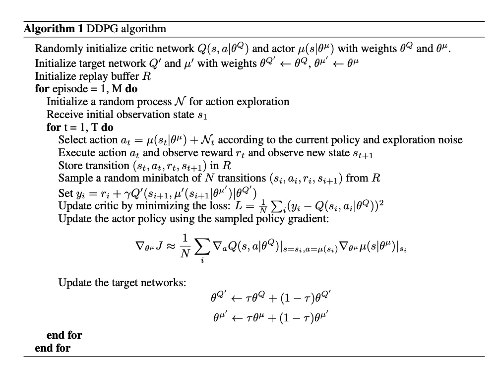
Pseudocode

\[ \begin{align}\begin{aligned}:nowrap:\\\begin{split}\begin{algorithm}[H] \caption{Deep Deterministic Policy Gradient} \label{alg1} \begin{algorithmic}[1] \STATE Input: initial policy parameters $\theta$, Q-function parameters $\phi$, empty replay buffer $\mathcal{D}$ \STATE Set target parameters equal to main parameters $\theta_{\text{targ}} \leftarrow \theta$, $\phi_{\text{targ}} \leftarrow \phi$ \REPEAT \STATE Observe state $s$ and select action $a = \text{clip}(\mu_{\theta}(s) + \epsilon, a_{Low}, a_{High})$, where $\epsilon \sim \mathcal{N}$ \STATE Execute $a$ in the environment \STATE Observe next state $s'$, reward $r$, and done signal $d$ to indicate whether $s'$ is terminal \STATE Store $(s,a,r,s',d)$ in replay buffer $\mathcal{D}$ \STATE If $s'$ is terminal, reset environment state. \IF{it's time to update} \FOR{however many updates} \STATE Randomly sample a batch of transitions, $B = \{ (s,a,r,s',d) \}$ from $\mathcal{D}$ \STATE Compute targets \begin{equation*} y(r,s',d) = r + \gamma (1-d) Q_{\phi_{\text{targ}}}(s', \mu_{\theta_{\text{targ}}}(s')) \end{equation*} \STATE Update Q-function by one step of gradient descent using \begin{equation*} \nabla_{\phi} \frac{1}{|B|}\sum_{(s,a,r,s',d) \in B} \left( Q_{\phi}(s,a) - y(r,s',d) \right)^2 \end{equation*} \STATE Update policy by one step of gradient ascent using \begin{equation*} \nabla_{\theta} \frac{1}{|B|}\sum_{s \in B}Q_{\phi}(s, \mu_{\theta}(s)) \end{equation*} \STATE Update target networks with \begin{align*} \phi_{\text{targ}} &\leftarrow \rho \phi_{\text{targ}} + (1-\rho) \phi \\ \theta_{\text{targ}} &\leftarrow \rho \theta_{\text{targ}} + (1-\rho) \theta \end{align*} \ENDFOR \ENDIF \UNTIL{convergence} \end{algorithmic} \end{algorithm}\end{split}\end{aligned}\end{align} \]

Extensions

DDPG can be combined with:

• Target Network

  Continuous control with deep reinforcement learning proposes soft target updates used to keep the network training stable. Since we implement soft update Target Network for actor-critic through TargetNetworkWrapper in model_wrap and configuring learn.target_theta.

• Initial collection of replay buffer following random policy

  Before optimizing the model parameters, we need to have a sufficient number of transition data in the replay buffer following random policy to ensure that the model does not overfit the replay buffer data at the beginning of the algorithm. So we control the number of transitions in the initial replay buffer by configuring random_collect_size. DDPG/TD3 random_collect_size is set to 25000 by default, while it is 10000 for SAC. We only simply follow SpinningUp default setting and use random policy to collect initialization data.

• Gaussian noise during collecting transition

  For the exploration noise process DDPG uses temporally correlated noise in order to generate temporally correlated exploration for exploration efficiency in physical control problems with inertia. Specifically, DDPG uses Ornstein-Uhlenbeck process with \(\theta = 0.15\) and \(\sigma = 0.2\). The Ornstein-Uhlenbeck process models the velocity of a Brownian particle with friction, which results in temporally correlated values centered around 0. However, we use Gaussian noise instead of Ornstein-Uhlenbeck noise due to too many hyper-parameters of Ornstein-Uhlenbeck noise. We configure collect.noise_sigma to control the exploration.

Implementations

The default config is defined as follows:

class ding.policy.ddpg.DDPGPolicy(cfg: easydict.EasyDict, model: Optional[torch.nn.modules.module.Module] = None, enable_field: Optional[List[str]] = None)

Overview:

Policy class of DDPG algorithm. Paper link: https://arxiv.org/abs/1509.02971.

Config:

ID	Symbol	Type	Default Value	Description	Other(Shape)
1	type	str	ddpg	RL policy register name, refer to registry POLICY_REGISTRY	this arg is optional, a placeholder
2	cuda	bool	False	Whether to use cuda for network
3	random_ collect_size	int	25000	Number of randomly collected training samples in replay buffer when training starts.	Default to 25000 for DDPG/TD3, 10000 for sac.
4	model.twin_ critic	bool	False	Whether to use two critic networks or only one.	Default False for DDPG, Clipped Double Q-learning method in TD3 paper.
5	learn.learning _rate_actor	float	1e-3	Learning rate for actor network(aka. policy).
6	learn.learning _rate_critic	float	1e-3	Learning rates for critic network (aka. Q-network).
7	learn.actor_ update_freq	int	2	When critic network updates once, how many times will actor network update.	Default 1 for DDPG, 2 for TD3. Delayed Policy Updates method in TD3 paper.
8	learn.noise	bool	False	Whether to add noise on target network’s action.	Default False for DDPG, True for TD3. Target Policy Smoo- thing Regularization in TD3 paper.
9	learn.- ignore_done	bool	False	Determine whether to ignore done flag.	Use ignore_done only in halfcheetah env.
10	learn.- target_theta	float	0.005	Used for soft update of the target network.	aka. Interpolation factor in polyak aver- aging for target networks.
11	collect.- noise_sigma	float	0.1	Used for add noise during co- llection, through controlling the sigma of distribution	Sample noise from dis- tribution, Ornstein- Uhlenbeck process in DDPG paper, Gaussian process in ours.

Model

Here we provide examples of ContinuousQAC model as default model for DDPG.

class ding.model.ContinuousQAC(obs_shape: Union[int, ding.utils.type_helper.SequenceType], action_shape: Union[int, ding.utils.type_helper.SequenceType, easydict.EasyDict], action_space: str, twin_critic: bool = False, actor_head_hidden_size: int = 64, actor_head_layer_num: int = 1, critic_head_hidden_size: int = 64, critic_head_layer_num: int = 1, activation: Optional[torch.nn.modules.module.Module] = ReLU(), norm_type: Optional[str] = None, encoder_hidden_size_list: Optional[ding.utils.type_helper.SequenceType] = None, share_encoder: Optional[bool] = False)

Overview:

The neural network and computation graph of algorithms related to Q-value Actor-Critic (QAC), such as DDPG/TD3/SAC. This model now supports continuous and hybrid action space. The ContinuousQAC is composed of four parts: actor_encoder, critic_encoder, actor_head and critic_head. Encoders are used to extract the feature from various observation. Heads are used to predict corresponding Q-value or action logit. In high-dimensional observation space like 2D image, we often use a shared encoder for both actor_encoder and critic_encoder. In low-dimensional observation space like 1D vector, we often use different encoders.

Interfaces:

__init__, forward, compute_actor, compute_critic

compute_actor(obs: torch.Tensor) → Dict[str, Union[torch.Tensor, Dict[str, torch.Tensor]]]

Overview:

QAC forward computation graph for actor part, input observation tensor to predict action or action logit.

Arguments:

• x (torch.Tensor): The input observation tensor data.

Returns:

• outputs (Dict[str, Union[torch.Tensor, Dict[str, torch.Tensor]]]): Actor output dict varying from action_space: regression, reparameterization, hybrid.

ReturnsKeys (regression):

• action (torch.Tensor): Continuous action with same size as action_shape, usually in DDPG/TD3.

ReturnsKeys (reparameterization):

• logit (Dict[str, torch.Tensor]): The predictd reparameterization action logit, usually in SAC. It is a list containing two tensors: mu and sigma. The former is the mean of the gaussian distribution, the latter is the standard deviation of the gaussian distribution.

ReturnsKeys (hybrid):

• logit (torch.Tensor): The predicted discrete action type logit, it will be the same dimension as action_type_shape, i.e., all the possible discrete action types.

• action_args (torch.Tensor): Continuous action arguments with same size as action_args_shape.

Shapes:

• obs (torch.Tensor): \((B, N0)\), B is batch size and N0 corresponds to obs_shape.

• action (torch.Tensor): \((B, N1)\), B is batch size and N1 corresponds to action_shape.

• logit.mu (torch.Tensor): \((B, N1)\), B is batch size and N1 corresponds to action_shape.

• logit.sigma (torch.Tensor): \((B, N1)\), B is batch size.

• logit (torch.Tensor): \((B, N2)\), B is batch size and N2 corresponds to action_shape.action_type_shape.

• action_args (torch.Tensor): \((B, N3)\), B is batch size and N3 corresponds to action_shape.action_args_shape.

Examples:

>>> # Regression mode
>>> model = ContinuousQAC(64, 6, 'regression')
>>> obs = torch.randn(4, 64)
>>> actor_outputs = model(obs,'compute_actor')
>>> assert actor_outputs['action'].shape == torch.Size([4, 6])
>>> # Reparameterization Mode
>>> model = ContinuousQAC(64, 6, 'reparameterization')
>>> obs = torch.randn(4, 64)
>>> actor_outputs = model(obs,'compute_actor')
>>> assert actor_outputs['logit'][0].shape == torch.Size([4, 6])  # mu
>>> actor_outputs['logit'][1].shape == torch.Size([4, 6]) # sigma

compute_critic(inputs: Dict[str, torch.Tensor]) → Dict[str, torch.Tensor]

Overview:

QAC forward computation graph for critic part, input observation and action tensor to predict Q-value.

Arguments:

• inputs (Dict[str, torch.Tensor]): The dict of input data, including obs and action tensor, also contains logit and action_args tensor in hybrid action_space.

ArgumentsKeys:

• obs: (torch.Tensor): Observation tensor data, now supports a batch of 1-dim vector data.

• action (Union[torch.Tensor, Dict]): Continuous action with same size as action_shape.

• logit (torch.Tensor): Discrete action logit, only in hybrid action_space.

• action_args (torch.Tensor): Continuous action arguments, only in hybrid action_space.

Returns:

• outputs (Dict[str, torch.Tensor]): The output dict of QAC’s forward computation graph for critic, including q_value.

ReturnKeys:

• q_value (torch.Tensor): Q value tensor with same size as batch size.

Shapes:

• obs (torch.Tensor): \((B, N1)\), where B is batch size and N1 is obs_shape.

• logit (torch.Tensor): \((B, N2)\), B is batch size and N2 corresponds to action_shape.action_type_shape.

• action_args (torch.Tensor): \((B, N3)\), B is batch size and N3 corresponds to action_shape.action_args_shape.

• action (torch.Tensor): \((B, N4)\), where B is batch size and N4 is action_shape.

• q_value (torch.Tensor): \((B, )\), where B is batch size.

Examples:

>>> inputs = {'obs': torch.randn(4, 8), 'action': torch.randn(4, 1)}
>>> model = ContinuousQAC(obs_shape=(8, ),action_shape=1, action_space='regression')
>>> assert model(inputs, mode='compute_critic')['q_value'].shape == (4, )  # q value

forward(inputs: Union[torch.Tensor, Dict[str, torch.Tensor]], mode: str) → Dict[str, torch.Tensor]

Overview:

QAC forward computation graph, input observation tensor to predict Q-value or action logit. Different mode will forward with different network modules to get different outputs and save computation.

Arguments:

• inputs (Union[torch.Tensor, Dict[str, torch.Tensor]]): The input data for forward computation graph, for compute_actor, it is the observation tensor, for compute_critic, it is the dict data including obs and action tensor.

• mode (str): The forward mode, all the modes are defined in the beginning of this class.

Returns:

• output (Dict[str, torch.Tensor]): The output dict of QAC forward computation graph, whose key-values vary in different forward modes.

Examples (Actor):

>>> # Regression mode
>>> model = ContinuousQAC(64, 6, 'regression')
>>> obs = torch.randn(4, 64)
>>> actor_outputs = model(obs,'compute_actor')
>>> assert actor_outputs['action'].shape == torch.Size([4, 6])
>>> # Reparameterization Mode
>>> model = ContinuousQAC(64, 6, 'reparameterization')
>>> obs = torch.randn(4, 64)
>>> actor_outputs = model(obs,'compute_actor')
>>> assert actor_outputs['logit'][0].shape == torch.Size([4, 6])  # mu
>>> actor_outputs['logit'][1].shape == torch.Size([4, 6]) # sigma

Examples (Critic):

>>> inputs = {'obs': torch.randn(4, 8), 'action': torch.randn(4, 1)}
>>> model = ContinuousQAC(obs_shape=(8, ),action_shape=1, action_space='regression')
>>> assert model(inputs, mode='compute_critic')['q_value'].shape == (4, )  # q value

Train actor-critic model

First, we initialize actor and critic optimizer in _init_learn, respectively. Setting up two separate optimizers can guarantee that we only update actor network parameters and not critic network when we compute actor loss, vice versa.

# actor and critic optimizer
self._optimizer_actor = Adam(
    self._model.actor.parameters(),
    lr=self._cfg.learn.learning_rate_actor,
    weight_decay=self._cfg.learn.weight_decay
)
self._optimizer_critic = Adam(
    self._model.critic.parameters(),
    lr=self._cfg.learn.learning_rate_critic,
    weight_decay=self._cfg.learn.weight_decay
)

In _forward_learn we update actor-critic policy through computing critic loss, updating critic network, computing actor loss, and updating actor network.

1. critic loss computation

   • current and target value computation

   # current q value
   q_value = self._learn_model.forward(data, mode='compute_critic')['q_value']
   # target q value. SARSA: first predict next action, then calculate next q value
   with torch.no_grad():
       next_action = self._target_model.forward(next_obs, mode='compute_actor')['action']
       next_data = {'obs': next_obs, 'action': next_action}
       target_q_value = self._target_model.forward(next_data, mode='compute_critic')['q_value']
   

   • loss computation

   # DDPG: single critic network
   td_data = v_1step_td_data(q_value, target_q_value, reward, data['done'], data['weight'])
   critic_loss, td_error_per_sample = v_1step_td_error(td_data, self._gamma)
   loss_dict['critic_loss'] = critic_loss
   

2. critic network update

self._optimizer_critic.zero_grad()
loss_dict['critic_loss'].backward()
self._optimizer_critic.step()

1. actor loss

actor_data = self._learn_model.forward(data['obs'], mode='compute_actor')
actor_data['obs'] = data['obs']
actor_loss = -self._learn_model.forward(actor_data, mode='compute_critic')['q_value'].mean()
loss_dict['actor_loss'] = actor_loss

1. actor network update

# actor update
self._optimizer_actor.zero_grad()
actor_loss.backward()
self._optimizer_actor.step()

Target Network

We implement Target Network trough target model initialization in _init_learn. We configure learn.target_theta to control the interpolation factor in averaging.

# main and target models
self._target_model = copy.deepcopy(self._model)
self._target_model = model_wrap(
    self._target_model,
    wrapper_name='target',
    update_type='momentum',
    update_kwargs={'theta': self._cfg.learn.target_theta}
)

Benchmark

environment	best mean reward	evaluation results	config link	comparison
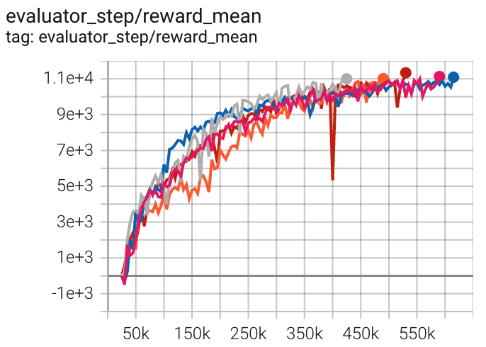
HalfCheetah (HalfCheetah-v3)	11334		config_link_p	Tianshou(11719) Spinning-up(11000)
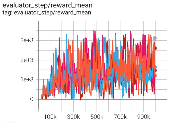
Hopper (Hopper-v2)	3516		config_link_q	Tianshou(2197) Spinning-up(1800)
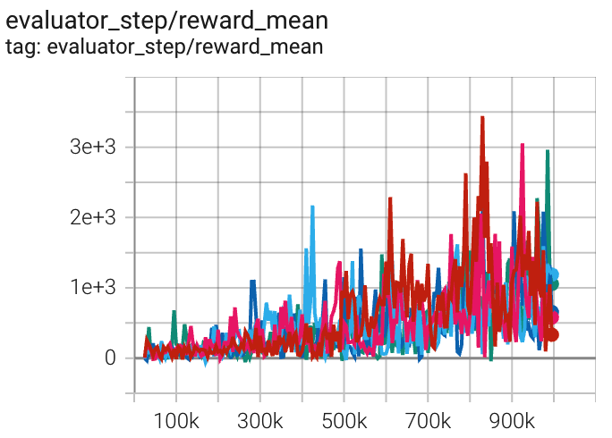
Walker2d (Walker2d-v2)	3443		config_link_s	Tianshou(1401) Spinning-up(1950)

P.S.:

1. The above results are obtained by running the same configuration on five different random seeds (0, 1, 2, 3, 4)

References

Timothy P. Lillicrap, Jonathan J. Hunt, Alexander Pritzel, Nicolas Heess, Tom Erez, Yuval Tassa, David Silver, Daan Wierstra: “Continuous control with deep reinforcement learning”, 2015; [http://arxiv.org/abs/1509.02971 arXiv:1509.02971].

David Silver, Guy Lever, Nicolas Heess, Thomas Degris, Daan Wierstra, et al.. Deterministic Policy Gradient Algorithms. ICML, Jun 2014, Beijing, China. ffhal-00938992f

Hafner, R., Riedmiller, M. Reinforcement learning in feedback control. Mach Learn 84, 137–169 (2011).

Degris, T., White, M., and Sutton, R. S. (2012b). Linear off-policy actor-critic. In 29th International Conference on Machine Learning.

Other Public Implementations

• Baselines

• sb3

• rllab

• rllib (Ray)

• TD3 release repo

• Spinningup

• tianshou