IMPALA¶

Overview¶

IMPALA, or the Importance Weighted Actor Learner Architecture, is an off-policy actor-critic framework that decouples data collecting from learning and optimizes policy from experience trajectories using off-policy correction V-trace. This method is firstly introduced in IMPALA: Scalable Distributed Deep-RL with Importance Weighted Actor-Learner Architectures.

Quick Facts¶

IMPALA is a model-free and off-policy RL algorithm.
IMPALA can support both discrete action spaces and continuous action spaces.
IMPALA is an actor-critic RL algorithm with value network, which optimizes actor network and critic (value) network, respectively.
IMPALA can take advantage of the old off-policy data with corresponding off-policy correction to stabilize learning.
IMPALA decouples data collecting from learning. Collectors in IMPALA will not compute value or advantage.
IMPALA is a distributed RL architecture with classic actor-learner paradigm.

Key Equations¶

Loss used in IMPALA is similar to that in PPO, A2C and other value function actor-critic models. All of them come from policy_loss,value_loss and entropy_loss, with respect to some carefully chosen weights, i.e.:

\[loss_{total} = loss_{policy} + w_{value} * loss_{value} + w_{entropy} * loss_{entropy}\]

Tip

NOTATION AND CONVENTIONS:

\(\pi_{\phi}\): current training policy parameterized by \(\phi\).

\(V_\theta\): value function parameterized by \(\theta\).

\(\mu\): older policy which generates trajectories in replay buffer.

At the training time \(t\), given transition \((x_t, a_t, x_{t+1}, r_t)\), the value function \(V_\theta\) is learned through an \(L_2\) loss between the current value and a V-trace target value. The n-step V-trace target at time s is defined as follows:

\[v_s \stackrel{def}{=} V(x_s) + \sum_{t=s}^{s+n-1} \gamma^{t-s} \big(\prod_{i=s}^{t-1} c_i\big)\delta_t V\]

where \(\delta_t V \stackrel{def}{=} \rho_t (r_t + \gamma V(x_{t+1}) - V(x_t))\) is a temporal difference for \(V\), \(\rho_t \stackrel{def}{=} \min\big(\bar{\rho}, \frac{\pi(a_t \vert x_t)}{\mu(a_t \vert x_t)}\big)\), and \(c_i \stackrel{def}{=}\min\big(\bar{c}, \frac{\pi(a_i \vert s_i)}{\mu(a_i \vert s_i)}\big)\)

\(\rho_t\) and \(c_i\) are truncated importance sampling (IS) weights, where \(\bar{\rho}\) and \(\bar{c}\) are two truncation constants with \(\bar{\rho} \geq \bar{c}\).

The product of \(c_s, \dots, c_{t-1}\) measures how much a temporal difference \(\delta_t V\) observed at time \(t\) impacts the update of the value function at a previous time \(s\) . In the on-policy case, we have \(\rho_t=1\) and \(c_i=1\) (assuming \(\bar{c} \geq 1)\) and therefore the V-trace target becomes on-policy n-step Bellman target.

Note

\(\bar{\rho}\) impacts the fixed-point of the value function we converge to, and \(\bar{c}\) impacts the speed of convergence.

When \(\bar{\rho} =\infty\) (untruncated), v-trace value function will converge to the value function of the target policy \(V_\pi\);

When \(\bar{\rho}\) is close to 0, we evaluate the value function of the behavior policy \(V_\mu\); when in-between, we evaluate a policy between \(\pi\) and \(\mu\).

Therefore, loss functions are

\[\begin{split}loss_{value} &= (v_s - V_\theta(x_s))^2 \\ loss_{policy} &= -\rho_s \log \pi_\phi(a_s \vert x_s) \big(r_s + \gamma v_{s+1} - V_\theta(x_s)\big) \\ loss_{entropy} &= -H(\pi_\phi) = \sum_a \pi_\phi(a\vert x_s)\log \pi_\phi(a\vert x_s)\end{split}\]

where \(H(\pi_{\phi})\), entropy of policy \(\phi\), is a bonus to encourage exploration.

Value function parameter is updated in the direction of:

\[\Delta\theta = w_{value} (v_s - V_\theta(x_s))\nabla_\theta V_\theta(x_s)\]

Policy parameter \(\phi\) is updated through policy gradient,

\[\begin{split}\Delta \phi &= \rho_s \nabla_\phi \log \pi_\phi(a_s \vert x_s) \big(r_s + \gamma v_{s+1}- V_\theta(x_s)\big)\\ &- w_{entropy} \nabla_\phi \sum_a \pi_\phi(a\vert x_s)\log \pi_\phi(a\vert x_s)\end{split}\]

where \(r_s + \gamma v_{s+1}\) is the v-trace advantage, which is estimated Q value subtracted by a state-dependent baseline \(V_\theta(x_s)\).

Key Graphs¶

The following graph describes the distributed architecture in IMPALA original paper. However, our implication is a little different from that in original paper.

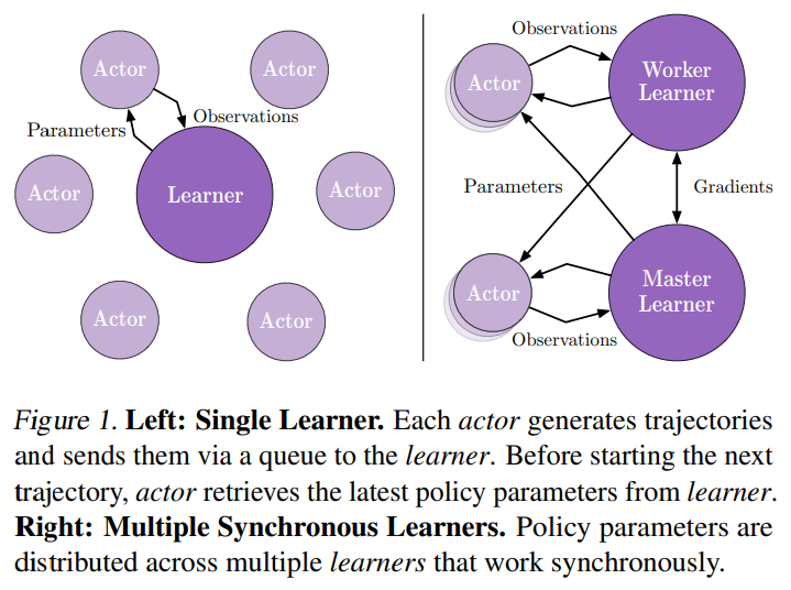
For single learner, they use multiple actors/collectors to generate training data. While in our setting, we use one collector which has multiple environments to increase data diversity.

For multiple learner, in original paper, different learners will have different actors with them. In other word, they will have different ReplayBuffer. While in our setting, all of the learners, will share the same ReplayBuffer, and will synchronize after each iteration.

Implementations¶

Config¶

The default config is defined as follows:

class ding.policy.impala.IMPALAPolicy(cfg: easydict.EasyDict, model: Optional[torch.nn.modules.module.Module] = None, enable_field: Optional[List[str]] = None)[source]¶

Overview:

Policy class of IMPALA algorithm. Paper link: https://arxiv.org/abs/1802.01561.

Config:

ID	Symbol	Type	Default Value	Description	Other(Shape)
1	`type`	str	impala	RL policy register name, refer to registry `POLICY_REGISTRY`	this arg is optional, a placeholder
2	`cuda`	bool	False	Whether to use cuda for network	this arg can be diff- erent from modes
3	`on_policy`	bool	False	Whether the RL algorithm is on-policy or off-policy
	`priority`	bool	False	Whether use priority(PER)	priority sample, update priority
5	`priority_` `IS_weight`	bool	False	Whether use Importance Sampling Weight	If True, priority must be True
6	`unroll_len`	int	32	trajectory length to calculate v-trace target
7	`learn.update` `per_collect`	int	4	How many updates(iterations) to train after collector’s one collection. Only valid in serial training	this args can be vary from envs. Bigger val means more off-policy

The network interface IMPALA used is defined as follows:

class ding.model.template.vac.VAC(obs_shape: Union[int, ding.utils.type_helper.SequenceType], action_shape: Union[int, ding.utils.type_helper.SequenceType, easydict.EasyDict], action_space: str = 'discrete', share_encoder: bool = True, encoder_hidden_size_list: ding.utils.type_helper.SequenceType = [128, 128, 64], actor_head_hidden_size: int = 64, actor_head_layer_num: int = 1, critic_head_hidden_size: int = 64, critic_head_layer_num: int = 1, activation: Optional[torch.nn.modules.module.Module] = ReLU(), norm_type: Optional[str] = None, sigma_type: Optional[str] = 'independent', fixed_sigma_value: Optional[int] = 0.3, bound_type: Optional[str] = None, encoder: Optional[torch.nn.modules.module.Module] = None, impala_cnn_encoder: bool = False)[source]
Overview:
The neural network and computation graph of algorithms related to (state) Value Actor-Critic (VAC), such as A2C/PPO/IMPALA. This model now supports discrete, continuous and hybrid action space. The VAC is composed of four parts: actor_encoder, critic_encoder, actor_head and critic_head. Encoders are used to extract the feature from various observation. Heads are used to predict corresponding value or action logit. In high-dimensional observation space like 2D image, we often use a shared encoder for both actor_encoder and critic_encoder. In low-dimensional observation space like 1D vector, we often use different encoders.

Interfaces:
__init__, forward, compute_actor, compute_critic, compute_actor_critic.
forward(x: torch.Tensor, mode: str) → Dict[source]
Overview:
VAC forward computation graph, input observation tensor to predict state value or action logit. Different mode will forward with different network modules to get different outputs and save computation.

Arguments:

x (torch.Tensor): The input observation tensor data.

mode (str): The forward mode, all the modes are defined in the beginning of this class.

Returns:

outputs (Dict): The output dict of VAC’s forward computation graph, whose key-values vary from different mode.

Examples (Actor):
>>> model = VAC(64, 128)
>>> inputs = torch.randn(4, 64)
>>> actor_outputs = model(inputs,'compute_actor')
>>> assert actor_outputs['logit'].shape == torch.Size([4, 128])
Examples (Critic):
>>> model = VAC(64, 64)
>>> inputs = torch.randn(4, 64)
>>> critic_outputs = model(inputs,'compute_critic')
>>> assert actor_outputs['logit'].shape == torch.Size([4, 64])
Examples (Actor-Critic):
>>> model = VAC(64, 64)
>>> inputs = torch.randn(4, 64)
>>> outputs = model(inputs,'compute_actor_critic')
>>> assert critic_outputs['value'].shape == torch.Size([4])
>>> assert outputs['logit'].shape == torch.Size([4, 64])

Data Processing¶

Usually, we hope to compute everything as a batch to improve efficiency. Especially, when computing vtrace, we need all training sample (sequences of training data) have the same length. This is done in policy._get_train_sample. Once we execute this function in collector, the length of samples will equal to unroll_len in config. For details, please refer to doc of ding.rl_utils.adder.

def _get_train_sample(self, data: List[Dict[str, Any]]) -> List[Dict[str, Any]]:
    return get_train_sample(data, self._unroll_len)

def get_train_sample(cls, data: List[Dict[str, Any]], unroll_len: int, last_fn_type: str = 'last') -> List[Dict[str, Any]]:
    """
    Overview:
        Process raw traj data by updating keys ['next_obs', 'reward', 'done'] in data's dict element.
        If ``unroll_len`` equals to 1, which means no process is needed, can directly return ``data``.
        Otherwise, ``data`` will be split according to ``self._unroll_len``, process residual part according to
        ``last_fn_type`` and call ``lists_to_dicts`` to form sampled training data.
    Arguments:
        - data (:obj:`List[Dict[str, Any]]`): transitions list, each element is a transition dict
    Returns:
        - data (:obj:`List[Dict[str, Any]]`): transitions list processed after unrolling
    """
    if unroll_len == 1:
        return data
    else:
        # cut data into pieces whose length is unroll_len
        split_data, residual = list_split(data, step=self._unroll_len)

        def null_padding():
            template = copy.deepcopy(residual[0])
            template['done'] = True
            template['reward'] = torch.zeros_like(template['reward'])
            if 'value_gamma' in template:
                template['value_gamma'] = 0.
            null_data = [cls._get_null_transition(template) for _ in range(miss_num)]
            return null_data

        if residual is not None:
            miss_num = unroll_len - len(residual)
            if last_fn_type == 'drop':
                # drop the residual part
                pass
            elif last_fn_type == 'last':
                if len(split_data) > 0:
                    # copy last datas from split_data's last element, and insert in front of residual
                    last_data = copy.deepcopy(split_data[-1][-miss_num:])
                    split_data.append(last_data + residual)
                else:
                    # get null transitions using ``null_padding``, and insert behind residual
                    null_data = null_padding()
                    split_data.append(residual + null_data)
            elif last_fn_type == 'null_padding':
                # same to the case of 'last' type and split_data is empty
                null_data = null_padding()
                split_data.append(residual + null_data)
        # collate unroll_len dicts according to keys
        if len(split_data) > 0:
            split_data = [lists_to_dicts(d, recursive=True) for d in split_data]
        return split_data

Note

In get_train_sample, we introduce three ways to cut trajectory data into same-length pieces (length equal to unroll_len).

1. The first one is drop, this means after splitting trajectory data into small pieces, we simply throw away those with length smaller than unroll_len. This method is kind of naive and usually is not a good choice. Since in Reinforcement Learning, the last few data in an episode is usually very important, we can’t just throw away them.

2. The second method is last, which means if the total length trajectory is smaller than unroll_len, we will use zero padding. Else, we will use data from previous piece to pad residual piece. This method is set as default and recommended.

The last method null_padding is just zero padding, which is not vert efficient since many data will be null.

Optimization¶

Now, we introduce the computation of vtrace-value. First, we use the following functions to compute importance_weights.

def compute_importance_weights(target_output, behaviour_output, action, requires_grad=False):
    """
    Shapes:
        - target_output (:obj:`torch.FloatTensor`): :math:`(T, B, N)`, where T is timestep, B is batch size and\
            N is action dim
        - behaviour_output (:obj:`torch.FloatTensor`): :math:`(T, B, N)`
        - action (:obj:`torch.LongTensor`): :math:`(T, B)`
        - rhos (:obj:`torch.FloatTensor`): :math:`(T, B)`
    """

    grad_context = torch.enable_grad() if requires_grad else torch.no_grad()
    assert isinstance(action, torch.Tensor)
    device = action.device

    with grad_context:
        dist_target = torch.distributions.Categorical(logits=target_output)
        dist_behaviour = torch.distributions.Categorical(logits=behaviour_output)
        rhos = dist_target.log_prob(action) - dist_behaviour.log_prob(action)
        rhos = torch.exp(rhos)
        return rhos

After that, we clip importance weights based on constant \(\rho\) and \(c\) to get clipped_rhos, clipped_cs. Then we can compute vtrace value according to the following function. Notice, here bootstrap_values are just value function \(V(x_s)\) in vtrace definition.

def vtrace_nstep_return(clipped_rhos, clipped_cs, reward, bootstrap_values, gamma=0.99, lambda_=0.95):
    """
    Shapes:
        - clipped_rhos (:obj:`torch.FloatTensor`): :math:`(T, B)`, where T is timestep, B is batch size
        - clipped_cs (:obj:`torch.FloatTensor`): :math:`(T, B)`
        - reward: (:obj:`torch.FloatTensor`): :math:`(T, B)`
        - bootstrap_values (:obj:`torch.FloatTensor`): :math:`(T+1, B)`
        - vtrace_return (:obj:`torch.FloatTensor`):  :math:`(T, B)`
    """
    deltas = clipped_rhos * (reward + gamma * bootstrap_values[1:] - bootstrap_values[:-1])
    factor = gamma * lambda_
    result = bootstrap_values[:-1].clone()
    vtrace_item = 0.
    for t in reversed(range(reward.size()[0])):
        vtrace_item = deltas[t] + factor * clipped_cs[t] * vtrace_item
        result[t] += vtrace_item
    return result

Note

1. Bootstrap_values in this part need to have size (T+1,B), where T is timestep, B is batch size. The reason is that we need a sequence of training data with same-length vtrace value (this length is just the unroll_len in config). And in order to compute the last vtrace value in the sequence, we need at least one more target value. This is done using the next obs of the last transition in training data sequence.

2. Here we introduce a parameter lambda_, following the implementation in AlphaStar. The parameter, between 0 and 1, can give a subtle control on vtrace off-policy correction. Usually, we will choose this parameter close to 1.

Once we get vtrace value, or vtrace_nstep_return, the computation of loss functions are straightforward. The whole process is as follows.

def vtrace_advantage(clipped_pg_rhos, reward, return_, bootstrap_values, gamma):
    """
    Shapes:
        - clipped_pg_rhos (:obj:`torch.FloatTensor`): :math:`(T, B)`, where T is timestep, B is batch size
        - reward: (:obj:`torch.FloatTensor`): :math:`(T, B)`
        - return_ (:obj:`torch.FloatTensor`):  :math:`(T, B)`
        - bootstrap_values (:obj:`torch.FloatTensor`): :math:`(T, B)`
        - vtrace_advantage (:obj:`torch.FloatTensor`):  :math:`(T, B)`
    """
    return clipped_pg_rhos * (reward + gamma * return_ - bootstrap_values)

def vtrace_error(
        data: namedtuple,
        gamma: float = 0.99,
        lambda_: float = 0.95,
        rho_clip_ratio: float = 1.0,
        c_clip_ratio: float = 1.0,
        rho_pg_clip_ratio: float = 1.0):
    """
    Shapes:
        - target_output (:obj:`torch.FloatTensor`): :math:`(T, B, N)`, where T is timestep, B is batch size and\
            N is action dim
        - behaviour_output (:obj:`torch.FloatTensor`): :math:`(T, B, N)`
        - action (:obj:`torch.LongTensor`): :math:`(T, B)`
        - value (:obj:`torch.FloatTensor`): :math:`(T+1, B)`
        - reward (:obj:`torch.LongTensor`): :math:`(T, B)`
        - weight (:obj:`torch.LongTensor`): :math:`(T, B)`
    """

    target_output, behaviour_output, action, value, reward, weight = data
    with torch.no_grad():
        IS = compute_importance_weights(target_output, behaviour_output, action)
        rhos = torch.clamp(IS, max=rho_clip_ratio)
        cs = torch.clamp(IS, max=c_clip_ratio)
        return_ = vtrace_nstep_return(rhos, cs, reward, value, gamma, lambda_)
        pg_rhos = torch.clamp(IS, max=rho_pg_clip_ratio)
        return_t_plus_1 = torch.cat([return_[1:], value[-1:]], 0)
        adv = vtrace_advantage(pg_rhos, reward, return_t_plus_1, value[:-1], gamma)

    if weight is None:
        weight = torch.ones_like(reward)
    dist_target = torch.distributions.Categorical(logits=target_output)
    pg_loss = -(dist_target.log_prob(action) * adv * weight).mean()
    value_loss = (F.mse_loss(value[:-1], return_, reduction='none') * weight).mean()
    entropy_loss = (dist_target.entropy() * weight).mean()
    return vtrace_loss(pg_loss, value_loss, entropy_loss)

Note

The shape of value in input data should be (T+1, B), the reason is same as above Note.
Here we introduce a parameter rho_pg_clip_ratio, following the implementation in AlphaStar. This parameter, can give a subtle control on vtrace advantage. Usually, we will choose this parameter just same as rho_clip_ratio.

Difference between old and new pipeline¶

The way of task startup and the training component organization form is very different in old and new pipeline. In old pipeline, the training process is serial and intuitive, each part of the training is fully expressed in the main function. In new pipeline, each part of the training is encapsulated as a function. The training process is completed through function calls, and use ‘task.context’ to control the data transfer during the training process.

Meanwhile, the way of data slicing is different too. In new pipeline, data will be sliced by ‘unroll_len’ first, then randomly selected.

Benchmark¶

Benchmark and comparison of IMPALA algorithm¶
environment	best mean reward	config link	comparison
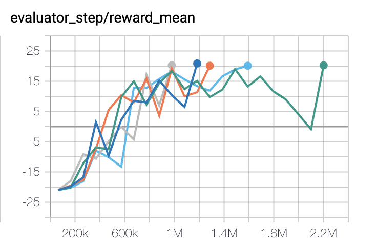
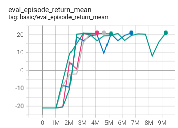
Pong (PongNoFrameskip-v4)	20	config_link_p	IMPALA paper shallow 200M (20.4)
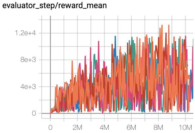
Qbert (QbertNoFrameskip-v4)	13175	config_link_q	IMPALA paper shallow 200M (18901)
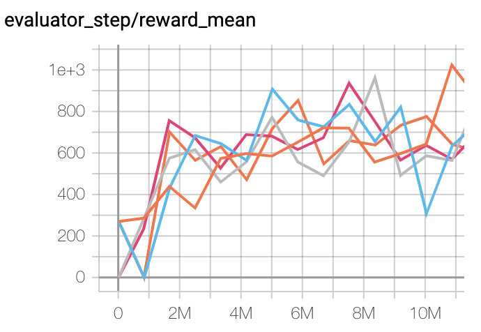
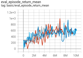
SpaceInvaders (SpaceInvadersNoFrame skip-v4)	977	config_link_s	IMPALA paper shallow 200M (1726)
Pong(In new pipeline) (Pong skip-v4)	21	config_link_np	IMPALA paper shallow 200M (20.4)
SpaceInvaders(In new pipeline) (SpaceInvadersNoFrame skip-v4)	1006	config_link_ns	IMPALA paper shallow 200M (1726)

P.S.：

The above results are obtained by running the same configuration on five different random seeds (0, 1, 2, 3, 4)
The environment with the in new pipeline suffix is trained using the new training process. The new training process is more concise and clear, and the data collection speed is faster.
For the discrete action space algorithm like IMPALA, the Atari environment set is generally used for testing (including sub-environments Pong), and Atari environment is generally evaluated by the highest mean reward training 10M env_step. For more details about Atari, please refer to Atari Env Tutorial .

Reference¶

Lasse Espeholt, Hubert Soyer, Remi Munos, Karen Simonyan, Volodymir Mnih, Tom Ward, Yotam Doron, Vlad Firoiu, Tim Harley, Iain Dunning, Shane Legg, Koray Kavukcuoglu: “IMPALA: Scalable Distributed Deep-RL with Importance Weighted Actor-Learner Architectures”, 2018; arXiv:1802.01561. https://arxiv.org/abs/1802.01561

Other Public Implementations¶

[Official](https://github.com/deepmind/scalable_agent)
[Facebook torchbeast](https://github.com/facebookresearch/torchbeast)