PPO
Overview
PPO (Proximal Policy Optimization) was proposed in Proximal Policy Optimization Algorithms. The key question to answer is that how can we utilize the existing data to take the most possible improvement step for the policy without accidentally leading to performance collapse. PPO follows the idea of TRPO (which restricts the step of policy update by explicit KL-divergence constraint), but doesn’t have a KL-divergence term in the objective, instead utilizing a specialized clipped objective to remove incentives for the new policy to get far from the old policy. PPO avoids the calculation of the Hessian matrix in TRPO, thus is simpler to implement and empirically performs at least as well as TRPO.
Quick Facts
PPO is a model-free and policy-gradient RL algorithm.
PPO supports both discrete and continuous action spaces.
PPO supports off-policy mode and on-policy mode.
PPO can be equipped with RNN.
PPO is a first-order gradient method that use a few tricks to keep new policies close to old.
Key Equations or Key Graphs
PPO use clipped probability ratios in the policy gradient to prevent the policy from too rapid changes, specifically the optimizing objective is:
where \(\frac{\pi_{\theta}(a \mid s)}{\pi_{\theta_{k}}(a \mid s)}\) is denoted as the probability ratio \(r_t(\theta)\), \(\theta\) are the policy parameters to be optimized at the current time, \(\theta_k\) are the parameters of the policy at iteration k and \(\gamma\) is a small hyperparameter control that controls the maximum update step size of the policy parameters.
According to this note, the PPO-Clip objective can be simplified to:
where,
Usually we don’t access to the true advantage value of the sampled state-action pair \((s,a)\), but luckily we can calculate a approximate value \(\hat{A}_t\). The idea behind this clipping objective is: for \((s,a)\), if \(\hat{A}_t < 0\), maximizing \(L^{C L I P}(\theta)\) means make \(\pi_{\theta}(a_{t} \mid s_{t})\) smaller, but no additional benefit to the objective function is gained by making \(\pi_{\theta}(a_{t} \mid s_{t})\) smaller than \((1-\epsilon)\pi_{\theta}(a_{t} \mid s_{t})\) . Analogously, if \(\hat{A}_t > 0\), maximizing \(L^{C L I P}(\theta)\) means make \(\pi_{\theta}(a_{t} \mid s_{t})\) larger, but no additional benefit is gained by making \(\pi_{\theta}(a_{t} \mid s_{t})\) larger than \((1+\epsilon)\pi_{\theta}(a_{t} \mid s_{t})\). Empirically, by optimizing this objective function, the update step of the policy network can be controlled within a reasonable range.
For the value function, in order to balance the bias and variance in value learning, PPO adopts the Generalized Advantage Estimator to compute the advantages, which is a exponentially-weighted sum of Bellman residual terms. that is analogous to TD(λ):
where V is an approximate value function, \(\delta_{t}=r_{t}+\gamma V\left(s_{t+1}\right)-V\left(s_{t}\right)\) is the Bellman residual terms, or called TD-error at timestep t.
The value target is calculated as: \(V_{t}^{target}=V_{t}+\hat{A}_{t}\), and the value loss is defined as a squared-error: \(\frac{1}{2}*\left(V_{\theta}\left(s_{t}\right)-V_{t}^{\mathrm{target}}\right)^{2}\), To ensure adequate exploration, PPO further enhances the objective by adding a policy entropy bonus.
The total PPO loss is a weighted sum of policy loss, value loss and policy entropy regularization term:
where c1 and c2 are coefficients that control the relative importance of different terms.
Note
The standard implementation of PPO contains the many additional optimizations which are not described in the paper. Further details can be found in IMPLEMENTATION MATTERS IN DEEP POLICY GRADIENTS: A CASE STUDY ON PPO AND TRPO.
Pseudo-code
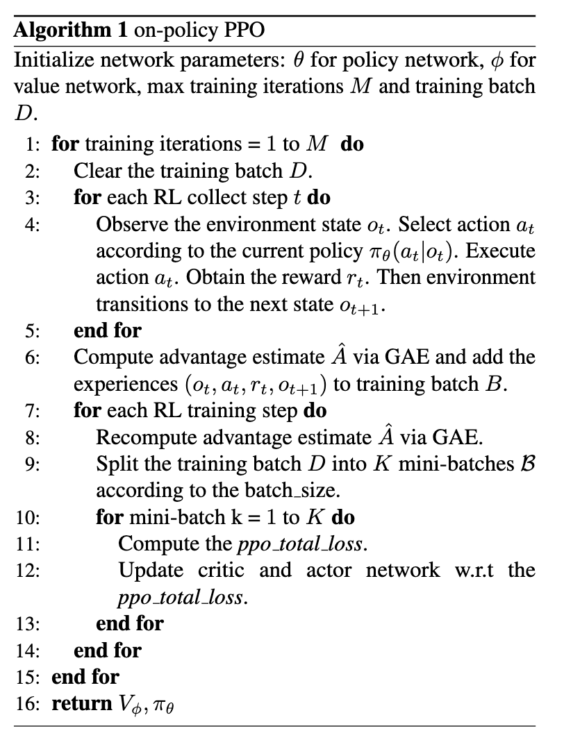
Note
This is the on-policy version of PPO. In DI-engine, we also have the off-policy version of PPO, which is almost the same as on-policy PPO except that we maintain a replay buffer that stored the recent experience, and the data used to calculate the PPO loss is sampled from the replay buffer not the recently collected batch, so off-policy PPO are able to reuse old data very efficiently, but potentially brittle and unstable.
Extensions
- PPO can be combined with:
Implementation
The default config is defined as follows:
- class ding.policy.ppo.PPOPolicy(cfg: EasyDict, model: Module | None = None, enable_field: List[str] | None = None)[source]
- Overview:
Policy class of on-policy version PPO algorithm. Paper link: https://arxiv.org/abs/1707.06347.
- class ding.model.template.vac.VAC(obs_shape: int | SequenceType, action_shape: int | SequenceType | EasyDict, action_space: str = 'discrete', share_encoder: bool = True, encoder_hidden_size_list: SequenceType = [128, 128, 64], actor_head_hidden_size: int = 64, actor_head_layer_num: int = 1, critic_head_hidden_size: int = 64, critic_head_layer_num: int = 1, activation: Module | None = ReLU(), norm_type: str | None = None, sigma_type: str | None = 'independent', fixed_sigma_value: int | None = 0.3, bound_type: str | None = None, encoder: Module | None = None, impala_cnn_encoder: bool = False)[source]
- Overview:
The neural network and computation graph of algorithms related to (state) Value Actor-Critic (VAC), such as A2C/PPO/IMPALA. This model now supports discrete, continuous and hybrid action space. The VAC is composed of four parts:
actor_encoder,critic_encoder,actor_headandcritic_head. Encoders are used to extract the feature from various observation. Heads are used to predict corresponding value or action logit. In high-dimensional observation space like 2D image, we often use a shared encoder for bothactor_encoderandcritic_encoder. In low-dimensional observation space like 1D vector, we often use different encoders.- Interfaces:
__init__,forward,compute_actor,compute_critic,compute_actor_critic.
- compute_actor(x: Tensor) Dict[source]
- Overview:
VAC forward computation graph for actor part, input observation tensor to predict action logit.
- Arguments:
x (
torch.Tensor): The input observation tensor data.- Returns:
outputs (
Dict): The output dict of VAC’s forward computation graph for actor, includinglogit.- ReturnsKeys:
logit (
torch.Tensor): The predicted action logit tensor, for discrete action space, it will be the same dimension real-value ranged tensor of possible action choices, and for continuous action space, it will be the mu and sigma of the Gaussian distribution, and the number of mu and sigma is the same as the number of continuous actions. Hybrid action space is a kind of combination of discrete and continuous action space, so the logit will be a dict withaction_typeandaction_args.- Shapes:
logit (
torch.Tensor): \((B, N)\), where B is batch size and N isaction_shape- Examples:
- compute_actor_critic(x: Tensor) Dict[source]
- Overview:
VAC forward computation graph for both actor and critic part, input observation tensor to predict action logit and state value.
- Arguments:
x (
torch.Tensor): The input observation tensor data.- Returns:
outputs (
Dict): The output dict of VAC’s forward computation graph for both actor and critic, includinglogitandvalue.- ReturnsKeys:
logit (
torch.Tensor): The predicted action logit tensor, for discrete action space, it will be the same dimension real-value ranged tensor of possible action choices, and for continuous action space, it will be the mu and sigma of the Gaussian distribution, and the number of mu and sigma is the same as the number of continuous actions. Hybrid action space is a kind of combination of discrete and continuous action space, so the logit will be a dict withaction_typeandaction_args.value (
torch.Tensor): The predicted state value tensor.- Shapes:
logit (
torch.Tensor): \((B, N)\), where B is batch size and N isaction_shapevalue (
torch.Tensor): \((B, )\), where B is batch size, (B, 1) is squeezed to (B, ).- Examples:
Note
compute_actor_criticinterface aims to save computation when shares encoder and return the combination dict output.
- compute_critic(x: Tensor) Dict[source]
- Overview:
VAC forward computation graph for critic part, input observation tensor to predict state value.
- Arguments:
x (
torch.Tensor): The input observation tensor data.- Returns:
outputs (
Dict): The output dict of VAC’s forward computation graph for critic, includingvalue.- ReturnsKeys:
value (
torch.Tensor): The predicted state value tensor.- Shapes:
value (
torch.Tensor): \((B, )\), where B is batch size, (B, 1) is squeezed to (B, ).- Examples:
- forward(x: Tensor, mode: str) Dict[source]
- Overview:
VAC forward computation graph, input observation tensor to predict state value or action logit. Different
modewill forward with different network modules to get different outputs and save computation.- Arguments:
x (
torch.Tensor): The input observation tensor data.mode (
str): The forward mode, all the modes are defined in the beginning of this class.- Returns:
outputs (
Dict): The output dict of VAC’s forward computation graph, whose key-values vary from differentmode.- Examples (Actor):
- Examples (Critic):
- Examples (Actor-Critic):
The policy loss and value loss of PPO is implemented as follows:
def ppo_error(
        data: namedtuple,
        clip_ratio: float = 0.2,
        use_value_clip: bool = True,
        dual_clip: Optional[float] = None
) -> Tuple[namedtuple, namedtuple]:

    assert dual_clip is None or dual_clip > 1.0, "dual_clip value must be greater than 1.0, but get value: {}".format(
        dual_clip
    )
    logit_new, logit_old, action, value_new, value_old, adv, return_, weight = data
    policy_data = ppo_policy_data(logit_new, logit_old, action, adv, weight)
    policy_output, policy_info = ppo_policy_error(policy_data, clip_ratio, dual_clip)
    value_data = ppo_value_data(value_new, value_old, return_, weight)
    value_loss = ppo_value_error(value_data, clip_ratio, use_value_clip)

    return ppo_loss(policy_output.policy_loss, value_loss, policy_output.entropy_loss), policy_info
The interface of ppo_policy_error and ppo_value_error is defined as follows:
- ding.rl_utils.ppo.ppo_policy_error(data: namedtuple, clip_ratio: float = 0.2, dual_clip: float | None = None, entropy_bonus: bool = True) Tuple[namedtuple, namedtuple][source]
- Overview:
Get PPO policy loss (both for classical RL in control/video games and LLM/VLM RLHF).
- Arguments:
data (
namedtuple): Ppo input data with fieids shown inppo_policy_data.clip_ratio (
float): Clip value for ratio, defaults to 0.2.dual_clip (
float): A parameter c mentioned in arXiv:1912.09729 Equ. 5, shoule be in [1, inf), defaults to 5.0, if you don’t want to use it, set this parameter to Noneentropy_bonus (
bool): Whether to use entropy bonus, defaults to True. LLM RLHF usually does not use it.- Returns:
ppo_policy_loss (
namedtuple): the ppo policy loss item, all of them are the differentiable 0-dim tensorppo_info (
namedtuple): the ppo optim information for monitoring, all of them are Python scalar- Shapes:
logit_new (
torch.FloatTensor): \((B, N)\), where B is batch size and N is action dimlogit_old (
torch.FloatTensor): \((B, N)\)action (
torch.LongTensor): \((B, )\)adv (
torch.FloatTensor): \((B, )\)weight (
torch.FloatTensororNone): \((B, )\)policy_loss (
torch.FloatTensor): \(()\), 0-dim tensorentropy_loss (
torch.FloatTensor): \(()\)- Examples:
Note
This function can be extended from B to more parallel dimensions, like (B, S), where S is the sequence length in LLM/VLM.
Note
For the action mask often used in LLM/VLM, users can set the weight to the action mask.
- ding.rl_utils.ppo.ppo_value_error(data: namedtuple, clip_ratio: float = 0.2, use_value_clip: bool = True) Tensor[source]
- Overview:
Get PPO value loss
- Arguments:
data (
namedtuple): ppo input data with fieids shown inppo_value_dataclip_ratio (
float): clip value for ratiouse_value_clip (
bool): whether use value clip- Returns:
value_loss (
torch.FloatTensor): the ppo value loss item, all of them are the differentiable 0-dim tensor- Shapes:
value_new (
torch.FloatTensor): \((B, )\), where B is batch sizevalue_old (
torch.FloatTensor): \((B, )\)return (
torch.FloatTensor): \((B, )\)weight (
torch.FloatTensororNone): \((B, )\)value_loss (
torch.FloatTensor): \(()\), 0-dim tensor- Examples:
Implementation Tricks
trick |
explanation |
|---|---|
Utilizing generalized advantage estimator to balance bias and variance in value learning.
|
|
the authors claim that when \(\hat{A}_t < 0\), a too large \(r_t(\theta)\) should also be clipped, which introduces dual clip:
\(\max \left(\min \left(r_{t}(\theta) \hat{A}_{t}, {clip}\left(r_{t}(\theta), 1-\epsilon, 1+\epsilon\right) \hat{A}_{t}\right), c \hat{A}_{t}\right)\)
|
|
In on-policy PPO, each time we collect a batch data, we will train many epochs to improve data efficiency.
And before the beginning of each training epoch, we recompute the advantage of historical transitions,
to keep the advantage is an approximate evaluation of current policy.
|
|
We standardize the targets of the value/advantage function using running estimates of the average
and standard deviation of the value/advantage targets. For more implementation details about
recompute advantage and normalization, users can refer to this discussion.
|
|
Value is clipped around the previous value estimates. We use the value clip_ratio same as that used to clip policy
probability ratios in the PPO policy loss function.
|
|
Using an orthogonal initialization scheme for the policy and value networks.
|
Benchmark
off-policy PPO Benchmark:
environment |
best mean reward |
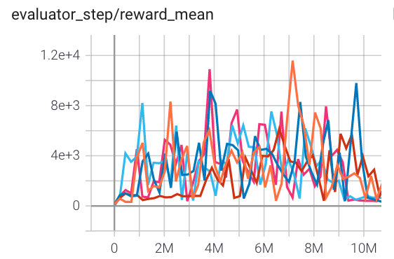
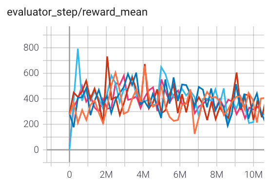
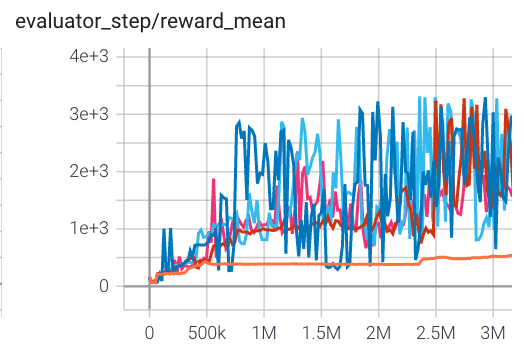
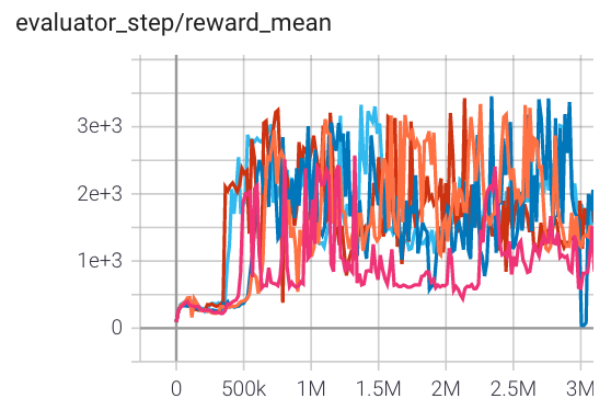
evaluation results |
config link |
comparison |
|---|---|---|---|---|
Pong (PongNoFrameskip-v4) |
20 |
|
||
Qbert (QbertNoFrameskip-v4) |
16400 |
|
||
SpaceInvaders (SpaceInvadersNoFrame skip-v4) |
1200 |

|
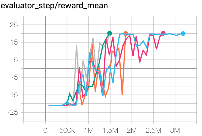
on-policy PPO Benchmark:
environment |
best mean reward |
evaluation results |
config link |
comparison |
|---|---|---|---|---|
Pong (PongNoFrameskip-v4) |
20 |
|
RLlib(20) |
|
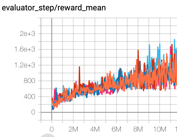
Qbert (QbertNoFrameskip-v4) |
12146 |
|
RLlib(11085) |
|
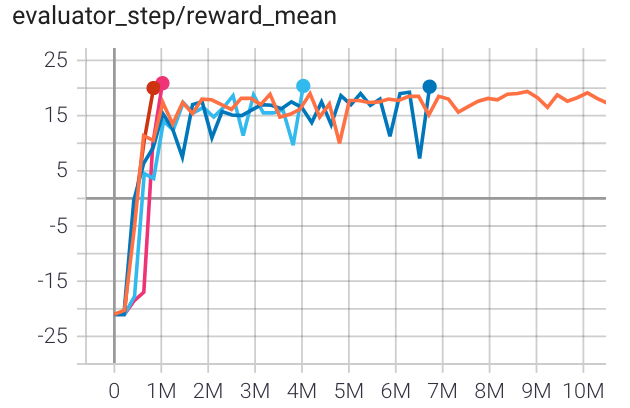
SpaceInvaders (SpaceInvadersNoFrame skip-v4) |
907 |
|
RLlib(671) |
|
Enduro (EnduroNoFrameskip- v4) |
957 |

|
RLlib(855) |
|
Hopper (Hopper-v3) |
3000 |
|
Tianshou(3127) Sb3(1567) spinningup(2500) |
|
Walker2d (Walker2d-v3) |
3700 |
|
Tianshou(4895) Sb3(1230) spinningup(2500) |
|
Halfcheetah (Halfcheetah-v3) |
3500 |
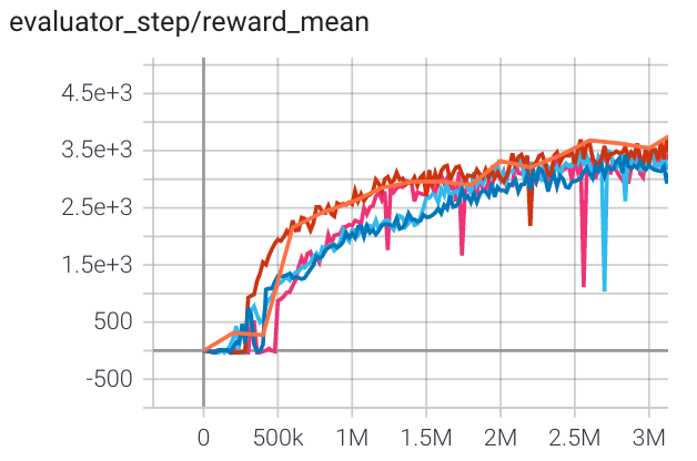
|
Tianshou(7337) Sb3(1976) spinningup(3000) |
|
Ant (Ant-v3) |
4200 |

|
Tianshou(3258) spinningup(650) |
References
John Schulman, Filip Wolski, Prafulla Dhariwal, Alec Radford, Oleg Klimov: “Proximal Policy Optimization Algorithms”, 2017; [http://arxiv.org/abs/1707.06347 arXiv:1707.06347].
Logan Engstrom, Andrew Ilyas, Shibani Santurkar, Dimitris Tsipras, Firdaus Janoos, Larry Rudolph, Aleksander Madry: “Implementation Matters in Deep Policy Gradients: A Case Study on PPO and TRPO”, 2020; [http://arxiv.org/abs/2005.12729 arXiv:2005.12729].
Andrychowicz M, Raichuk A, Stańczyk P, et al. What matters in on-policy reinforcement learning? a large-scale empirical study[J]. arXiv preprint arXiv:2006.05990, 2020.
Ye D, Liu Z, Sun M, et al. Mastering complex control in moba games with deep reinforcement learning[C]//Proceedings of the AAAI Conference on Artificial Intelligence. 2020, 34(04): 6672-6679.