Offline Reinforcement Learning¶

Problem Definition and Motivation¶

Offline Reinforcement Learning(RL), also known as Batch Reinforcement Learning, is a variant of RL that effectively leverages large, previously collected datasets for large-scale real-world applications. The use of static datasets means that during the training process of the agent, offline RL does not perform any form of online interaction and exploration, which is also the most significant difference from online reinforcement learning methods. For convenience, we refer to non-offline reinforcement learning, including both on-policy and off-policy RL, as online reinforcement learning (Online RL) in the following sections.

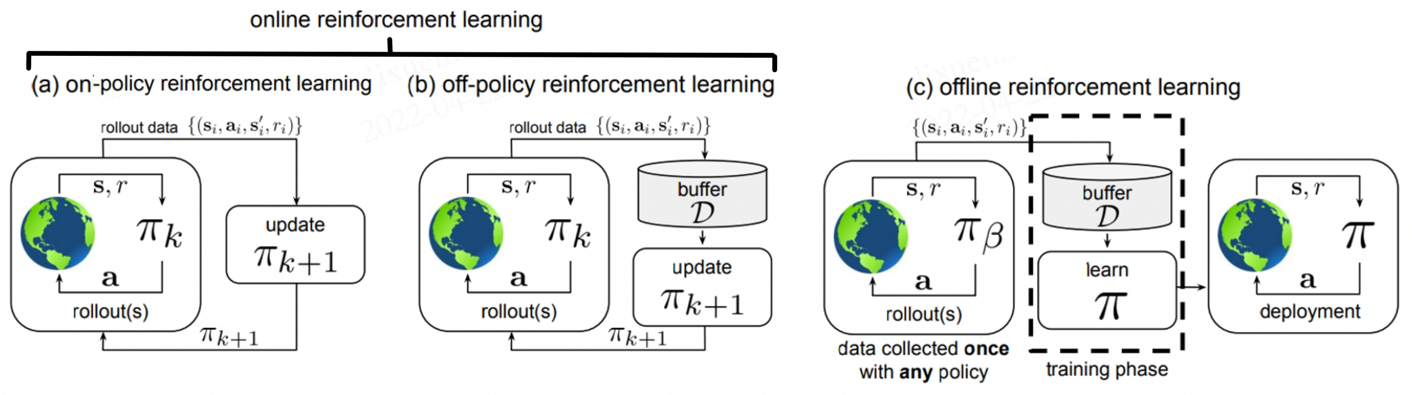
In the figure, (a) stands for On-policy RL, where the agent uses the current policy \(\pi_k\) to interact with the environment. Only data generated by currently learned policy can be used to update the network. (b) describes off-policy RL, which stores data of all historical policies in the experience buffer \(\mathcal{D}\) when interacting with the environment. In other words, \(\mathcal {D}\) contains data collected with policies \(\pi_0, \pi_1, ..., \pi_k\), and all of this will be used to update the network \(\pi_{k+ 1}\). For offline RL in (c), the dataset \(\mathcal{D}\) is collected from some (possibly unknown) behavioral policy \(\pi_{\beta}\) in advance, and will not change during training. The training process does not interact with the MDP at all, and the policy is only deployed after being fully trained.

Why Study Offline RL?

Offline RL has become a hot research topic recently, and the reasons can be attributed to two folds:

The first one is the advantage of offline RL itself. Deep reinforcement learning has achieved great success in simulation tasks such as games, and by effectively interacting with the environment, we can obtain agents with outstanding performance. However, it is usually too expensive to explore the environment and collect large-scale data for training repeatedly in real-world tasks. Especially it can be dangerous in environments such as autonomous driving and robotic operations. In contrast, offline RL studies how to learn an optimal policy from a fixed dataset, which can significantly mitigate potential risks and costs by not requiring any additional exploration.

Furthermore, the success of machine learning methods over the past decade can largely be attributed to the advent of scalable data-driven learning methods, which use more data to obtain better training results. Compared to online RL, taking full advantage of large-scale static datasets is also a significant advantage of offline RL.

Offline RL Training

Offline RL prohibits any kinds of interaction and exploration during training。 Under this setting, we train agents utilizing static dataset \(\mathcal{D}\), which is collected by some behavioral policy \(\pi_{\beta}(\mathbf{a}\mid \mathbf{s})\). Given \(\mathcal{D} = \left\{ (\mathbf{s}, \mathbf{a}, r, \mathbf{s}^{\prime})\right\}\), the value iteration and policy optimization process can be represented as:

\[\begin{split}\hat{Q}^{k+1} \leftarrow \arg\min_{Q} \mathbb{E}_{\mathbf{s}, \mathbf{a} \sim \mathcal{D}} \left[ \left(\hat{\mathcal{B}}^\pi \hat{Q}(\mathbf{s}, \mathbf{a}) - Q(\mathbf{s}, \mathbf{a}) \right)^2 \right], \\ \hat{\pi}^{k+1} \leftarrow \arg\max_{\pi} \mathbb{E}_{\mathbf{s} \sim \mathcal{D}, \mathbf{a} \sim \pi^{k}(\mathbf{a} \mid \mathbf{s})}\left[\hat{Q}^{k+1}(\mathbf{s}, \mathbf{a})\right],\end{split}\]

where the Bellman Operator \(\hat{\mathcal{B}}^\pi\) of policy \(\hat{\pi} \left(\mathbf{a} \mid \mathbf{s}\right)\) is \(\hat{\mathcal{B}}^\pi \hat{Q}\left(\mathbf{s}, \mathbf{a}\right) = \mathbb{E}_{\mathbf{s}, \mathbf{a}, \mathbf{s}^{\prime} \sim \mathcal{D}}[ r(\mathbf{s}, \mathbf{a})+\gamma \mathbb{E}_{\mathbf{a}^{\prime} \sim \hat{\pi}^{k}\left(\mathbf{a}^{\prime} \mid \mathbf{s}^{\prime}\right)}\left[\hat{Q}^{k}\left(\mathbf{s}^{\prime}, \mathbf{a}^{\prime}\right)\right] ]\).

Offline RL VS Imitation Learning

Offline RL is closely related to imitation learning (IL) in that the latter also learns from a fixed dataset without exploration. However, there are several key differences:

So far, offline RL algorithms have been built on top of standard off-policy Deep Reinforcement Learning (Deep RL) algorithms, which tend to optimize some form of a Bellman equation or TD difference error.
Most IL problems assume an optimal, or at least a high-performing, demonstrator which provides data, whereas offline RL may have to handle highly suboptimal data.
Most IL problems do not have a reward function. Offline RL considers rewards, which furthermore can be processed after-the-fact and modified.
Some IL problems require the data to be labeled as expert versus non-expert, while offline RL does not make this assumption.

Offline RL VS Off-policy RL

Off-policy RL generally refers to a class of RL algorithms that allow the policy which interacts with the environment to generate training samples to be different from the policy to be updated currently. Q-learning based algorithms, Actor-Critic algorithms that utilize Q-functions, and many Model-based RL algorithms belong to this category. Nevertheless, off-policy RL still often uses additional interactions (i.e. online data collection) during the learning process.

The Obstacle of Applying Online RL Algorithms to Offline Setting

Many previous research works have shown that online reinforcement learning algorithms perform poorly in offline RL scenarios. In paper [6], the author shows that it is because the policy tends to choose out-of-distribution actions (out-of-distribution, OOD). The estimation of the Q-function is accurate only when the distribution of the data to be estimated follows the distribution of training data. The relationship is shown in the following figure:

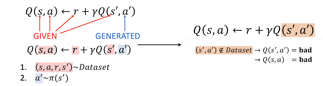
When the agent performs online exploration, the dataset is updated as well as the policy. The Markov static state distribution of the policy and the actual state distribution in the dataset is always the same (on-policy setting) or at least similar (off-policy setting). However, there will be a distributional shift compared to the original dataset in the offline scenario. During the expected reward maximization process, if the Q-function overestimates unseen \((\mathbf{s}, \mathbf{a})\) pairs, it is possible to select actions with low returns, resulting in poor performances.

Main Research Directions¶

Accoding to NeurIPS 2020 Tutorial 1 by Aviral Kumar and Sergey Levine, model-free offline RL could be classified as the following three categories:

Policy constraint methods
Uncertainty-based methods
Value regularization methods

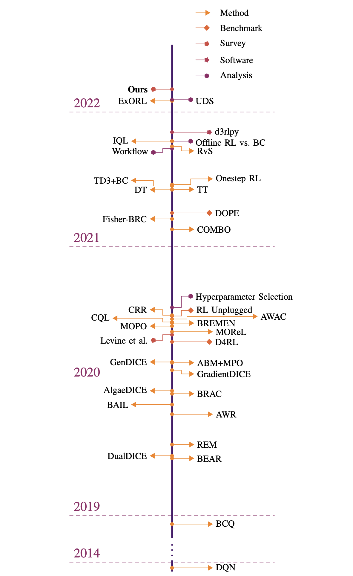
In addition, there are also works for Model-based RL in offline settings, which will not be carried out here. Interested readers can refer to 7 8 and other documents. For the overall development roadmap of offline RL, you can refer to the overview diagram in 9:

Policy Constraint Methods

This kind of method aims to keep learned policy \(\pi(\mathbf{a} \mid \mathbf{s})\) close enough to the behavioral policy \(\pi_{\beta}(\mathbf{a} \mid \mathbf{s})\), thus ensuring a precise Q-estimation. The distance between the aformentioned two policies could be represented as \(\mathbf{D}(\pi, \pi_{\beta})\)。In explicit constraints, the distance is constraint to be smaller than a specific value \(\mathcal{C}\),

\[\mathbf{D}_f(\pi, \pi_{\beta}) \le \mathcal{C}, \forall \pi\]

There are also implicit constraints such as policy reconstruction, mimicking the behavioral policy \(\pi_{\beta}(\mathbf{a} \mid \mathbf{s})\) with a trim level of perturbation. In BCQ 2, researchers propose to train a generative model (VAE) to simulate actions in the dataset. During the update process, the policy selects the action with the highest Q-value from the actions generated by the VAE perturbation, thereby ensuring that the selected action is similar to the action in the dataset. Based on BCQ, use TD3 as the network structure, then the TD3BC algorithm is derived. For details, please refer to 3.

Moreover, the distance \(\mathbf{D}(\pi, \pi_{\beta})\) could be regarded as a penalty term added to the objective or reward functions.

Uncertainty-based Methods

Aside from directly constraining the policy, we can also mitigate the effect of out-of-distribution actions by making the Q-function resilient to such queries, via effective uncertainty estimation. This kind of methods requires learning an uncertainty set or distribution \(\mathcal{P}(\mathbf{Q}^{\pi})\). Details are provided in 4 5. Then we can desgin a penalty term \(\mathcal{P}(\mathbf{Q}^{\pi})\) added to the Q-function.

\[\pi_{k+1} \leftarrow \arg\max_{\pi}\mathbb{E}_{\mathbf{s} \sim \mathcal{D}}[\mathbb{E}_{\mathbf{a} \sim \pi(\mathbf{a} \mid \mathbf{s})}[\mathbb{E}_{\mathbf{Q}_{k+1}^{\pi} \sim \mathcal{P}(\mathbf{Q}^{\pi})}[\mathbf{Q}_{k+1}^{\pi}(\mathbf{s}, \mathbf{a})] - \alpha \mathbf{Unc}(\mathcal{P}(\mathbf{Q}^{\pi}))]],\]

where \(\mathbf{Unc}(\cdot)\) denotes a metric of uncertainty, such that subtracting it provides a conservative estimate of the actual Q-function.

Value Regularization Methods

In CQL 6, a regularization term is plugged into the objective. This approach can be appealing for several reasons, such as being applicable to both actor-critic and Q-learning methods, even when a policy is not represented explicitly, and avoiding the need for explicit modeling of the behavior policy.

Similar to uncertainty-based method, CQL aims to derive a conservative Q-estimation.

\[\hat{\mathcal{E}}(\mathcal{B}, \mathcal{\phi}) = \alpha\mathcal{C}(\mathcal{B}, \mathcal{\phi}) + \mathcal{E}(\mathcal{B}, \mathbf{\phi}),\]

where the bellman error \(\mathcal{E}(\mathcal{B}, \mathcal{\phi})\) is the objective in classic DQN, and \(\mathcal{C}(\mathcal{B}, \mathcal{\phi})\) denotes the additional conservative penalty term. Different choices for \(\mathcal{C}(\mathcal{B}, \mathcal{\phi})\) lead to algorithms with different properties.

\[\mathcal{C}_{CQL_0}(\mathcal{B}, \mathbf{\phi}) = \mathbb{E}_{\mathbf{s} \sim \mathcal{D}}\mathbb{E}_{\mathbf{a} \sim \mu(\mathbf{a} \mid \mathbf{s})}[\mathbf{Q}_{\phi}(\mathbf{s}, \mathbf{a})],\]

the effect is that the conservative penalty will push down on high Q-values under some distribution \(\mu(\mathbf{a} \mid \mathbf{s})\). A simple and practical choice for \(\mu(\mathbf{a} \mid \mathbf{s})\) is:

\[\mu = \arg\max_{\mu} \mathbb{E}_{\mathbf{s} \sim \mathcal{D}}[\mathbb{E}_{\mathbf{a} \sim \mu(\mathbf{a} \mid \mathbf{s})}[\mathbf{Q}_{\phi}(\mathbf{s}, \mathbf{a})] + \mathcal{H}(\mu(\cdot \mid \mathbf{s}))],\]

The meaning is the policy that maximize the expected discounted return given the current data. Therefore, if the penalty weight \(\alpha\) is chosen appropriately, the conservative penalty should mostly push down on Q-values for out-of-distribution actions, since in-distribution actions would be “anchored” by the Bellman error \(\mathcal{E}(\mathcal{B}, \mathcal{\phi})\).

If \(\mathcal{C}_{CQL_0}(\mathcal{B}, \mathbf{\phi})\) is too conservative on the Q-estimation, we can choose

\[\mathcal{C}_{CQL_1}(\mathcal{B}, \mathbf{\phi}) = \mathbb{E}_{\mathbf{s} \sim \mathcal{D}}\mathbb{E}_{\mathbf{a} \sim \mu(\mathbf{a} \mid \mathbf{s})}[\mathbf{Q}_{\phi}(\mathbf{s}, \mathbf{a})] - \mathbb{E}_{(\mathbf{s}, \mathbf{a}) \sim \mathcal{D}}[\mathbf{Q}_{\phi}(\mathbf{s}, \mathbf{a})].\]

Future Outlooks¶

Standard off-policy RL algorithms have conventionally focused on dynamic programming methods that can utilize off-policy data. However, both of these classes of approaches struggle when coming to the fully offline condition. More recently, a number of improvements for ofﬂine RL methods have been proposed that take into account the statistics of the distributional shift via either policy constraints, uncertainty estimation, or value regularization. Generally speaking, such methods shed light on the fact that offline RL is actually a counter-factual inference problem: given data that resulted from a given set of decisions, infer the consequence of a different set of decisions. In conventional machine learning, we usually assume that the training and testing data are independently and identically distributed (i.i.d.). But offline RL drops this assumption, which is exceptionally challenging. To make this possible, new innovations are required to implement sophisticated statistical methods and combine them with the fundamentals of sequential decision-making in online RL. Methods such as solving distribution shifts, constraining action distribution, and evaluating the lower boundary of the distribution are all likely to achieve breakthroughs at the current offline RL research level.

In machine learning, a large part of the fantastic achievements of the past decade or so can be attributed to the data-driven learning paradigm. In computer vision and natural language, the increasing size and diversity of datasets have been an essential driver of progress despite the rapid performance gains driven by improvements in architectures and models, especially in real-world applications. Ofﬂine RL offers the possibility of turning reinforcement learning - which is conventionally viewed as a fundamentally active learning paradigm - into a data-driven discipline. However, in the standard setting of most online reinforcement learning methods, collecting large and diverse datasets is often impractical. The risks and costs are enormous in many applications, such as autonomous driving and human-computer interaction. Therefore, we look forward to witnessing a new generation of data-driven reinforcement learning in the future. It enables reinforcement learning not only to solve a range of real-world problems that were previously unsolvable, but also to take full advantage of larger, more diverse, and more expressive datasets in existing applications (driving, robotics, etc.).

Reference¶

1: Levine, S., A. Kumar, G. Tucker, and J. Fu (2020). Offline reinforcement learning: Tutorial, review, and perspectives on open problems. arXiv preprint arXiv:2005.01643.
2: Fujimoto, S., Meger, D., and Precup, D. (2018). Off-policy deep reinforcement learning without exploration. arXiv preprint arXiv:1812.02900.
3: Fujimoto, S., Gu, S. S. (2021). A Minimalist Approach to Offline Reinforcement Learning. arXiv preprint arXiv:2106.06860.
4: Jaksch, T., Ortner, R., and Auer, P. (2010). Near-optimal regret bounds for reinforcement learning. Journal of Machine Learning Research, 11(Apr):1563–1600.
5: O’Donoghue, B., Osband, I., Munos, R., and Mnih, V. (2018). The uncertainty bellman equation and exploration. In International Conference on Machine Learning, pages 3836–3845.
6: Kumar, A., Zhou, A., Tucker, G., and Levine, S. (2020b). Conservative q-learning for ofﬂine reinforcement learning. In Neural Information Processing Systems (NeurIPS).
7: Lerer, A., Gross, S., and Fergus, R. (2016). Learning physical intuition of block towers by example. arXiv preprint arXiv:1603.01312.
8: Battaglia, P., Pascanu, R., Lai, M., Rezende, D. J., et al. (2016). Interaction networks for learning about objects, relations and physics. In Advances in neural information processing systems, pages 4502–4510.
9: Rafael Figueiredo Prudencio, Marcos R. O. A. Maximo, Esther Luna Colombini. A Survey on Offline Reinforcement Learning: Taxonomy, Review, and Open Problems. CoRR abs/2203.01387 (2022)