RND
Overview
RND (Random Network Distillation) was first proposed in Exploration by Random Network Distillation , which introduces an exploration bonus for deep reinforcement learning methods that is easy to implement and adds minimal overhead to the computation performed. The exploration bonus is the error of a neural network predicting features of the observations given by a fixed randomly initialized neural network. RND claims that it is the first method that achieves better than average human performance on Montezuma’s Revenge without using demonstrations or having access to the underlying state of the game.
Quick Facts
The insight behind exploration approaches is that we first establish a method to measure the novelty of states, namely, how well we know this state, or the number of times we have visited a state similar to it. Then we assign a exploration reward in proportional to the novelty measure of the state. If the visited state is more novel, or say the state is explored very few times, the agent will get a bigger intrinsic reward. On the contrary, if the agent is more familiar with this state, or say, the state have been explored many times, the agent will get a smaller intrinsic reward on this state.
RND is a prediction-error-based exploration approach that can be applied in non-tabular cases. The main idea of prediction-error-based approaches is that defining the intrinsic reward as the prediction error for a problem related to the agent’s transitions, such as learning forward dynamics model, learning inverse dynamics model, or even a randomly generated problem, which is the case in RND algorithm.
RND involves two neural networks: a fixed and randomly initialized target network which sets the prediction problem, and a predictor network trained on data collected by the agent.
In RND paper, the underlying base RL algorithm is off-policy PPO. Generally, RND intrinsic reward generation model can be combined with many different RL algorithms such as DDPG, TD3, SAC conveniently.
Key Equations or Key Graphs
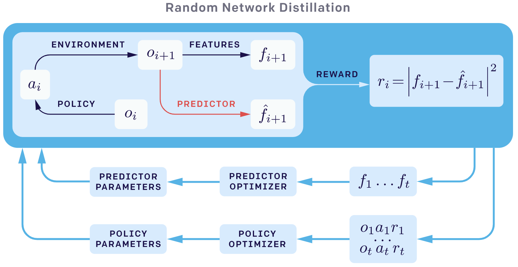
The following two graphs are from OpenAI’s blog. The overall sketch of RND is as follows:
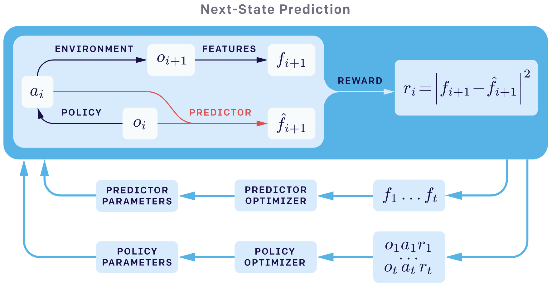
The overall sketch of next_sate_prediction exploration method is as follows:
In RND paper, the authors point out that prediction errors can be attributed to the following factors:
Amount of training data. Prediction error is high where few similar examples were seen by the predictor.
Stochasticity. Prediction error is high because the target function is stochastic. Stochastic transitions are a source of such error for forward dynamics prediction.
Model misspecification. Prediction error is high because information necessary for the prediction is missing, or the model class of predictors is too limited to fit the complexity of the target function.
Factor 1 is a useful source of error since it quantifies the novelty of experience, whereas factors 2 and 3 cause the noisy-TV problem, that is serious in the next_sate_prediction based exploration method. RND obviates factors 2 and 3 since the target network is chosen to be deterministic and has the identical network structure with the model-class of the predictor network.
In RND, the target network takes an observation to an embedding \(f: O → R^k\) and the predictor neural network \(\hat{f}: O → R^k\) is trained by gradient descent to minimize the expected MSE \(|f (x; θ) − f (x)|\) with respect to its parameters \(θ_\hat{f}\). In unfamiliar states it’s hard to predict the output of the fixed randomly initialized neural network, and hence the prediction error is higher, so RND can consider the prediction error as a measure of the novelty of visited states.
But RND is still facing some problems, one of which is that the RND bonus reward could gradually disappear over time, because with the training progresses advancing, the predictor network can fit the output of the randomly initialized neural network better and better. Interested readers can refer to the follow-up improvement work Never Give Up: Learning Directed Exploration Strategies and Agent57: Outperforming the Atari Human Benchmark.
The implementation details that matters
1. intrinsic reward normalization and weight factors. Normalize the intrinsic reward by the min-max normalization method, i.e., first minus the mini-batch min and divide it by the difference between the mini-batch max and the the mini-batch min. After the min-max normalization, the RND intrinsic reward is scaled into [0,1]. And we should also use some weight factor to control the balance of exploration and exploitation. For MiniGrid, in each episode, we let the last non-zero positive original reward times 1000 (more general, the weight factor could be the max length of the game) as the final fusion-reward to enlarge the effect of its original goal. And our experiment results in minigrid empty8 here shows that the balance of exploration and exploitation (here in exploration RL alg, i.e. the weight factor of intrinsic reward) is critical to achieve good performance in MiniGrid envs.
2. observation normalization. Whiten each dimension by subtracting the running mean and then dividing by the running standard deviation. Then clip the normalized observations to be between -5 and 5. Initialize the normalization parameters by stepping a random agent in the environment for a small number of steps before beginning optimization. Use the same observation normalization for both predictor and target networks but not the policy network.
3. Non-episodic intrinsic reward and two value heads. Non-episodic setting (which means the return is not truncated at “game over” status) resulted in more exploration than the episodic setting when exploring without any extrinsic rewards. In order to combine episodic and non-episodic reward streams, the rnd author recommend two value heads. When combing the episodic and non-episodic returns, a higher discount factor for the extrinsic rewards leads to better performance, while for intrinsic rewards it hurts exploration. So the rnd author recommend to set discount factor as 0.999 for extrinsic rewards and 0.99 for intrinsic rewards.
Note
In our implementation, for simplicity, we don’t adopt the following tricks: non-episodic intrinsic reward, two value heads and different discount factors.
In order to understand the reasons behind these tricks more clearly, it is recommended to read the original rnd paper .
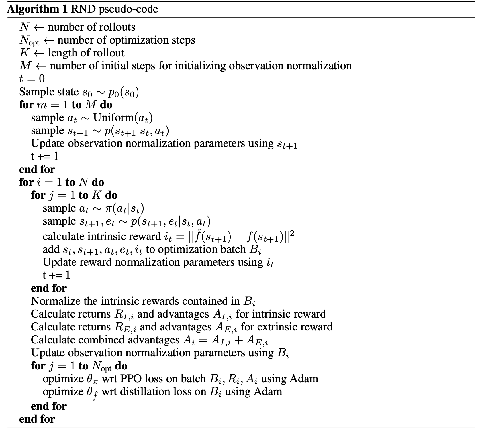
Pseudo-Code
Code Implementation
The interface of RND reward model is defined as follows:
- class ding.reward_model.rnd_reward_model.RndRewardModel(config: EasyDict, device: str = 'cpu', tb_logger: SummaryWriter = None)[source]
- Overview:
The RND reward model class (https://arxiv.org/abs/1810.12894v1)
- Interface:
estimate,train,collect_data,clear_data,__init__,_train,load_state_dict,state_dict- Config:
ID
Symbol
Type
Default Value
Description
Other(Shape)
1
typestr
rnd
Reward model register name, referto registryREWARD_MODEL_REGISTRY2
intrinsic_reward_typestr
add
the intrinsic reward typeincluding add, new, or assign3
learning_ratefloat
0.001
The step size of gradient descent4
batch_sizeint
64
Training batch size5
hidden_size_listlist (int)
[64, 64, 128]
the MLP layer shape6
update_per_collectint
100
Number of updates per collect7
obs_normbool
True
Observation normalization8
obs_norm_clamp_minint
0
min clip value for obs normalization9
obs_norm_clamp_maxint
1
max clip value for obs normalization10
intrinsic_reward_weightfloat
0.01
the weight of intrinsic rewardr = w*r_i + r_e11
extrinsic_reward_normbool
True
Whether to normlize extrinsic reward12
extrinsic_reward_norm_maxint
1
the upper bound of the rewardnormalization
- estimate(data: list) List[Dict][source]
Rewrite the reward key in each row of the data.
The interface of on policy PPO is defined as follows:
- class ding.policy.ppo.PPOPolicy(cfg: EasyDict, model: Module | None = None, enable_field: List[str] | None = None)[source]
- Overview:
Policy class of on-policy version PPO algorithm. Paper link: https://arxiv.org/abs/1707.06347.
Note: ... indicates the omitted code snippet. For the complete code, please refer to our
implementation in DI-engine.
RndNetwork
First, we define the class RndNetwork involves two neural networks: the fixed and randomly initialized target network self.target,
and the predictor network self.predictor trained on data collected by the agent.
class RndNetwork(nn.Module):

   def __init__(self, obs_shape: Union[int, SequenceType], hidden_size_list: SequenceType) -> None:
       super(RndNetwork, self).__init__()
       if isinstance(obs_shape, int) or len(obs_shape) == 1:
           self.target = FCEncoder(obs_shape, hidden_size_list)
           self.predictor = FCEncoder(obs_shape, hidden_size_list)
       elif len(obs_shape) == 3:
           self.target = ConvEncoder(obs_shape, hidden_size_list)
           self.predictor = ConvEncoder(obs_shape, hidden_size_list)
       else:
           raise KeyError(
               "not support obs_shape for pre-defined encoder: {}, please customize your own RND model".
               format(obs_shape)
           )
       for param in self.target.parameters():
           param.requires_grad = False

   def forward(self, obs: torch.Tensor) -> Tuple[torch.Tensor, torch.Tensor]:
       predict_feature = self.predictor(obs)
       with torch.no_grad():
           target_feature = self.target(obs)
       return predict_feature, target_feature
RndRewardModel
Then, we initialize reward model, optimizer and self._running_mean_std_rnd in _init_ of class RndRewardModel.
class RndRewardModel(BaseRewardModel):
    ...
    def __init__(self, config: EasyDict, device: str, tb_logger: 'SummaryWriter') -> None:  # noqa
       ...
       self.reward_model = RndNetwork(config.obs_shape, config.hidden_size_list)
       ...
       self.opt = optim.Adam(self.reward_model.predictor.parameters(), config.learning_rate)
       ...
       self._running_mean_std_rnd = RunningMeanStd(epsilon=1e-4)
Train RndRewardModel
Afterwards, we calculate the reward model loss and update the RND predictor network: self.reward_model.predictor. Note that, according to the
original paper, we adopt the observation normalization trick that is transforming the original observations to mean 0, std 1, and clip the normalized observations
to be between -5 and 5, which is empirically important especially when using a random network as a target, for the detailed explanation, please refer the chapter 2.4 in the RND paper.
def _train(self) -> None:
       train_data: list = random.sample(self.train_data, self.cfg.batch_size)
       train_data: torch.Tensor = torch.stack(train_data).to(self.device)

       # observation normalization:  transform to mean 0, std 1
       self._running_mean_std_rnd_obs.update(train_data.cpu().numpy())
       train_data = (train_data - to_tensor(self._running_mean_std_rnd_obs.mean)) / to_tensor(self._running_mean_std_rnd_obs.std)
       train_data = torch.clamp(train_data, min=-5, max=5)

       predict_feature, target_feature = self.reward_model(train_data)
       loss = F.mse_loss(predict_feature, target_feature.detach())
       self.opt.zero_grad()
       loss.backward()
       self.opt.step()
Calculate RND Reward
Finally, we calculate MSE loss according to the RND reward model and do the necessary subsequent processing
and rewrite the reward key in the data in estimate method of class RndRewardModel. And note that
we adapt the reward normalization trick that is transforming the original RND reward to (mean 0, std 1), empirically we found this normalization way works well
than only dividing the self._running_mean_std_rnd.std in some sparse reward environment, such as minigrid.
calculate the RND pseudo rewardobs = collect_states(data) obs = torch.stack(obs).to(self.device) # observation normalization: transform to mean 0, std 1 obs = (obs - to_tensor(self._running_mean_std_rnd_obs.mean)) / to_tensor(self._running_mean_std_rnd_obs.std) obs = torch.clamp(obs, min=-5, max=5) with torch.no_grad(): predict_feature, target_feature = self.reward_model(obs) reward = F.mse_loss(predict_feature, target_feature, reduction='none').mean(dim=1) self._running_mean_std_rnd.update(reward.cpu().numpy()) # reward normalization: transform to [0,1], empirically we found this normalization way works well # than only dividing the self._running_mean_std_rnd.std rnd_reward = (reward - reward.min()) / (reward.max() - reward.min() + 1e-11)2.
combine the RND pseudo reward with the original reward. Here, we should also use some weight factor to control the balance of exploration and exploitation. For minigrid, we let the last non-zero original reward times 1000 to enlarge the effect of original goal. We also conduct the experiment on minigrid empty8 to verify the importance of tradeoff between the exploration and exploitation. In the experiment, we found that if we don’t use the weight factor 1000, the rnd agent can’t learn to reach the goal at all because the proportion of exploration is too large.for item, rnd_rew in zip(data, reward): if self.intrinsic_reward_type == 'add': item['reward'] += rew if item['reward'] > 0 and item['reward'] <= 1: # for minigrid item['reward'] = 1000 * item['reward'] + rnd_rew else: item['reward'] += rnd_rew elif self.intrinsic_reward_type == 'new': item['intrinsic_reward'] = rnd_rew elif self.intrinsic_reward_type == 'assign': item['reward'] = rnd_rew
Benchmark Results
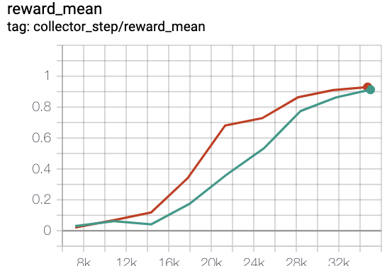
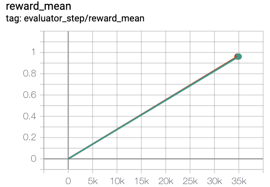
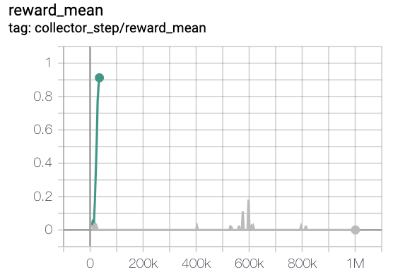
Because in collection phase, we use multinomial_sample to increase the diversity of collected data, in evaluation phase, we use the argmax action to interact with env, and we run 5 different seeds and report the mean reward. In the experimental results below, the x-axis denotes the total env-steps interacting with the env in the training process. In the graph labeled “collector_step”, the y-axis shows the rewards received during the collection phase, denoted as collect_reward; in the graph labeled “evaluator_step”, the y-axis shows the rewards obtained during the evaluation phase, denoted as episode_return. In the sparse reward envs minigrid, only when the agent reach the goal, the agent will get a positive reward, zero otherwise, and its value will be inversely proportional to the steps used to reach the goal. In the easiest env MiniGrid-Empty-8x8-v0, different seeds will have the same room configurations, the optimal reward is about 0.96. But in MiniGrid-FourRooms-v0, different seeds will have different room configurations and corresponding optimal reward is also different, when the mean of episode_return is greater than 0.6, we consider the env have been solved.
MiniGrid-Empty-8x8-v0(40k env steps,episode return_mean>0.95)
green line is rnd-onppo-weight100
red line is onppo
green line is rnd-onppo-weight100
grey line is rnd-onppo-noweight
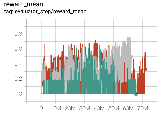
MiniGrid-FourRooms-v0(20M env steps,episode return_mean>0.6)
red line is onppo
grey line is rnd-onppo-weight1000
green line is rnd-onppo-weight100
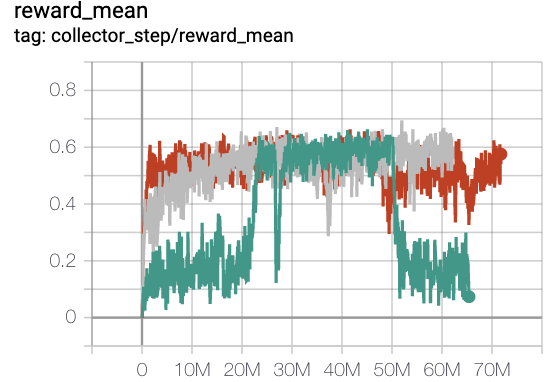
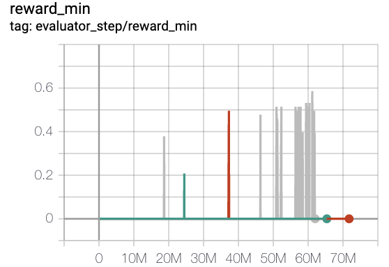
We can found that in rnd using the weight factor 1000 is much better than using 100. We hypothesis that it’s due to the episode length needed in fourrooms to solve the game is larger than in empty8 on average, so the total cumulated discounted intrinsic rewards in fourrooms is larger than in empty8. we should make sure the original reward to be comparable with intrinsic reward to trade-off between exploitation and exploration. This reminds us that the weight factor of original reward should be related to the total time-steps of solving the game.
Note
How to determine the relative weight between the intrinsic reward and the original extrinsic reward can be valuable work in the future.
Reference
Burda Y, Edwards H, Storkey A, et al. Exploration by random network distillation[J]. https://arxiv.org/abs/1810.12894v1. arXiv:1810.12894, 2018.
https://openai.com/blog/reinforcement-learning-with-prediction-based-rewards/