SAC¶

Overview¶

Soft actor-critic (SAC) is a stable and efficient model-free off-policy maximum entropy actor-critic algorithm for continuous state and action spaces, which is proposed in the 2018 paper Soft Actor-Critic: Off-Policy Maximum Entropy Deep Reinforcement Learning with a Stochastic Actor. The augmented entropy objective of the policy brings a number of conceptual and practical advantages including a more powerful exploration and the ability of the policy to capture multiple modes of near optimal behavior. The authors also showed that this method by combining off-policy updates with a stable stochastic actor-critic formulation, achieves state-of-the-art performance on a range of continuous control benchmark tasks, outperforming prior on-policy and off-policy methods.

Quick Facts¶

SAC is implemented for environments with continuous action spaces.(i.e. MuJoCo, Pendulum, and LunarLander)
SAC is an off-policy and model-free algorithm, combined with non-empty replay buffer for policy exploration.
SAC is a actor-critic RL algorithm, which optimizes actor network and critic network, respectively,
SAC is also implemented for multi-continuous action space.

Key Equations or Key Graphs¶

SAC considers a more general maximum entropy objective, which favors stochastic policies by augmenting the objective with the expected entropy of the policy:

\[J(\pi)=\sum_{t=0}^{T} \mathbb{E}_{\left(\mathbf{s}_{t}, \mathbf{a}_{t}\right) \sim \rho_{\pi}}\left[r\left(\mathbf{s}_{t}, \mathbf{a}_{t}\right)+\alpha \mathcal{H}\left(\pi\left(\cdot \mid \mathbf{s}_{t}\right)\right)\right].\]

The temperature parameters \(\alpha > 0\) controls the stochasticity of the optimal policy.

Soft Actor-Critic: Off-Policy Maximum Entropy Deep Reinforcement Learning with a Stochastic Actor considers a parameterized state value function, soft Q-function, and a tractable policy. Specifically, the value function and the soft Q-function are modeled as expressive neural networks, and the policy as a Gaussian with mean and covariance given by neural networks. In particular, SAC applies the reparameterization trick instead of directly minimizing the expected KL-divergence for policy parameters as

\[J_{\pi}(\phi)=\mathbb{E}_{\mathbf{s}_{t} \sim \mathcal{D}, \epsilon_{t} \sim \mathcal{N}}\left[\log \pi_{\phi}\left(f_{\phi}\left(\epsilon_{t} ; \mathbf{s}_{t}\right) \mid \mathbf{s}_{t}\right)-Q_{\theta}\left(\mathbf{s}_{t}, f_{\phi}\left(\epsilon_{t} ; \mathbf{s}_{t}\right)\right)\right]\]

We implement reparameterization trick through configuring learn.reparameterization.

Note

Compared with the vanilla version modeling state value function and soft Q-function, our implementation contains two versions. One is modeling state value function and soft Q-function, the other is only modeling soft Q-function through double network.

Note

Soft Actor-Critic: Off-Policy Maximum Entropy Deep Reinforcement Learning with a Stochastic Actor considers a parameterized state value function, soft Q-function, and a tractable policy. Our implementation contains two versions. One is modeling state value function and soft Q-function, the other is only modeling soft Q-function through double network. We configure model.value_network, model.twin_q, and learn.learning_rate_value to switch implementation version.

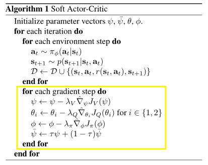
Pseudocode¶

Note

Compared with the vanilla version, we only optimize q network and actor network in our second implementation version.

Extensions¶

SAC can be combined with:

Auto alpha strategy

Reinforcement Learning with Deep Energy-Based Policies proposes entropy coefficient \(\alpha\) used to determine the relative importance of entropy and reward. Extensive experiments conducted by Soft Actor-Critic: Off-Policy Maximum Entropy Deep Reinforcement Learning with a Stochastic Actor demonstrate Soft actor-critic is sensitive to reward scaling since it is related to the temperature of the optimal policy. The optimal reward scale varies between environments, and should be tuned for each task separately. Since we implement auto alpha strategy depending on maximum entropy through configuring learn.is_auto_alpha and learn.alpha.

Implementation¶

The default config is defined as follows:

class ding.policy.sac.SACPolicy(cfg: easydict.EasyDict, model: Optional[torch.nn.modules.module.Module] = None, enable_field: Optional[List[str]] = None)[source]¶

Overview:

Policy class of continuous SAC algorithm. Paper link: https://arxiv.org/pdf/1801.01290.pdf

Config:

ID	Symbol	Type	Default Value	Description	Other
1	`type`	str	sac	RL policy register name, refer to registry `POLICY_REGISTRY`	this arg is optional, a placeholder
2	`cuda`	bool	True	Whether to use cuda for network
3	`on_policy`	bool	False	SAC is an off-policy algorithm.
4	`priority`	bool	False	Whether to use priority sampling in buffer.
5	`priority_IS_` `weight`	bool	False	Whether use Importance Sampling weight to correct biased update
6	`random_` `collect_size`	int	10000	Number of randomly collected training samples in replay buffer when training starts.	Default to 10000 for SAC, 25000 for DDPG/ TD3.
7	`learn.learning` `_rate_q`	float	3e-4	Learning rate for soft q network.	Defalut to 1e-3
8	`learn.learning` `_rate_policy`	float	3e-4	Learning rate for policy network.	Defalut to 1e-3
9	`learn.alpha`	float	0.2	Entropy regularization coefficient.	alpha is initiali- zation for auto alpha, when auto_alpha is True
10	`learn.` `auto_alpha`	bool	False	Determine whether to use auto temperature parameter alpha.	Temperature parameter determines the relative importance of the entropy term against the reward.
11	`learn.-` `ignore_done`	bool	False	Determine whether to ignore done flag.	Use ignore_done only in env like Pendulum
12	`learn.-` `target_theta`	float	0.005	Used for soft update of the target network.	aka. Interpolation factor in polyak aver aging for target networks.

We take the second version implementation (only predict soft Q function) as an example to introduce SAC algorithm:

Basic Actor-Critic Definition

Initialization Model.

# build network
self._policy_net = PolicyNet(self._obs_shape, self._act_shape, self._policy_embedding_size)

self._twin_q = twin_q
if not self._twin_q:
    self._soft_q_net = SoftQNet(self._obs_shape, self._act_shape, self._soft_q_embedding_size)
else:
    self._soft_q_net = nn.ModuleList()
    for i in range(2):
        self._soft_q_net.append(SoftQNet(self._obs_shape, self._act_shape, self._soft_q_embedding_size))

Soft Q prediction from soft Q network

def compute_critic_q(self, inputs: Dict[str, torch.Tensor]) -> Dict[str, torch.Tensor]:
    action = inputs['action']
    if len(action.shape) == 1:
        action = action.unsqueeze(1)
    state_action_input = torch.cat([inputs['obs'], action], dim=1)
    q_value = self._soft_q_net_forward(state_action_input)
    return {'q_value': q_value}

Action prediction from policy network

def compute_actor(self, obs: torch.Tensor, deterministic_eval=False, epsilon=1e-6) -> Dict[str, torch.Tensor]:
    mean, log_std = self._policy_net_forward(obs)
    std = log_std.exp()

    # unbounded Gaussian as the action distribution.
    dist = Independent(Normal(mean, std), 1)
    # for reparameterization trick (mean + std * N(0,1))
    if deterministic_eval:
        x = mean
    else:
        x = dist.rsample()
    y = torch.tanh(x)
    action = y

    # epsilon is used to avoid log of zero/negative number.
    y = 1 - y.pow(2) + epsilon
    log_prob = dist.log_prob(x).unsqueeze(-1)
    log_prob = log_prob - torch.log(y).sum(-1, keepdim=True)

    return {'mean': mean, 'log_std': log_std, 'action': action, 'log_prob': log_prob}

Note

SAC applys an invertible squashing function to the Gaussian samples, and employ the change of variables formula to compute the likelihoods of the bounded actions. Specifically, we use unbounded Gaussian as the action distribution through Independent(Normal(mean, std), 1), which creates a diagonal Normal distribution with the same shape as a Multivariate Normal distribution. This is equal to log_prob.sum(axis=-1). Then, the action is squashed by \(\tanh(\text{mean})\), and the log-likelihood of action has a simple form \(\log \pi(\mathbf{a} \mid \mathbf{s})=\log \mu(\mathbf{u} \mid \mathbf{s})-\sum_{i=1}^{D} \log \left(1-\tanh ^{2}\left(u_{i}\right)\right)\). In particular, the std in SAC is predicted from observation, which is different from PPO(learnable parameter) and TD3(heuristic parameter).

Entropy-Regularized Reinforcement Learning as follows

Entropy in target q value.

# target q value. SARSA: first predict next action, then calculate next q value
with torch.no_grad():
    (mu, sigma) = self._learn_model.forward(next_obs, mode='compute_actor')['logit']

    dist = Independent(Normal(mu, sigma), 1)
    pred = dist.rsample()
    next_action = torch.tanh(pred)
    y = 1 - next_action.pow(2) + 1e-6
    # keep dimension for loss computation (usually for action space is 1 env. e.g. pendulum)
    next_log_prob = dist.log_prob(pred).unsqueeze(-1)
    next_log_prob = next_log_prob - torch.log(y).sum(-1, keepdim=True)

    next_data = {'obs': next_obs, 'action': next_action}
    target_q_value = self._target_model.forward(next_data, mode='compute_critic')['q_value']
    # the value of a policy according to the maximum entropy objective
    if self._twin_critic:
        # find min one as target q value
        target_q_value = torch.min(target_q_value[0],
                                   target_q_value[1]) - self._alpha * next_log_prob.squeeze(-1)
    else:
        target_q_value = target_q_value - self._alpha * next_log_prob.squeeze(-1)

Soft Q value network update.

# =================
# q network
# =================
# compute q loss
if self._twin_q:
    q_data0 = v_1step_td_data(q_value[0], target_value, reward, done, data['weight'])
    loss_dict['q_loss'], td_error_per_sample0 = v_1step_td_error(q_data0, self._gamma)
    q_data1 = v_1step_td_data(q_value[1], target_value, reward, done, data['weight'])
    loss_dict['q_twin_loss'], td_error_per_sample1 = v_1step_td_error(q_data1, self._gamma)
    td_error_per_sample = (td_error_per_sample0 + td_error_per_sample1) / 2
else:
    q_data = v_1step_td_data(q_value, target_value, reward, done, data['weight'])
    loss_dict['q_loss'], td_error_per_sample = v_1step_td_error(q_data, self._gamma)

# update q network
self._optimizer_q.zero_grad()
loss_dict['q_loss'].backward()
if self._twin_q:
    loss_dict['q_twin_loss'].backward()
self._optimizer_q.step()

Entropy in policy loss.

# compute policy loss
policy_loss = (self._alpha * log_prob - new_q_value.unsqueeze(-1)).mean()

loss_dict['policy_loss'] = policy_loss

# update policy network
self._optimizer_policy.zero_grad()
loss_dict['policy_loss'].backward()
self._optimizer_policy.step()

Note

We implement reparameterization trick trough \((\text{mean} + \text{std} * \mathcal{N}(0,1))\). In particular, the gradient back propagation for sigma is through log_prob in policy loss.

Auto alpha strategy

Alpha initialization through log action shape.

if self._cfg.learn.is_auto_alpha:
    self._target_entropy = -np.prod(self._cfg.model.action_shape)
    self._log_alpha = torch.log(torch.tensor([self._cfg.learn.alpha]))
    self._log_alpha = self._log_alpha.to(device='cuda' if self._cuda else 'cpu').requires_grad_()
    self._alpha_optim = torch.optim.Adam([self._log_alpha], lr=self._cfg.learn.learning_rate_alpha)
    self._is_auto_alpha = True
    assert self._log_alpha.shape == torch.Size([1]) and self._log_alpha.requires_grad
    self._alpha = self._log_alpha.detach().exp()

Alpha update.

# compute alpha loss
if self._is_auto_alpha:
    log_prob = log_prob.detach() + self._target_entropy
    loss_dict['alpha_loss'] = -(self._log_alpha * log_prob).mean()

    self._alpha_optim.zero_grad()
    loss_dict['alpha_loss'].backward()
    self._alpha_optim.step()
    self._alpha = self._log_alpha.detach().exp()

Benchmark¶

environment

best mean reward

evaluation results

config link

comparison

Halfcheetah

(Halfcheetah-v3)

12900

config_link_ha

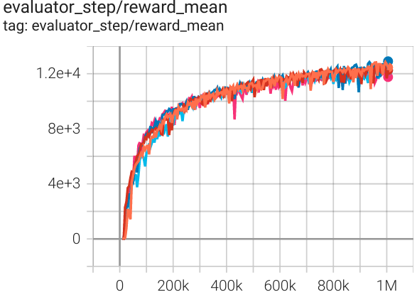
Spinning Up (13000)

SB3(9535)

Tianshou(12138)

Walker2d

(Walker2d-v2)

5172

config_link_w

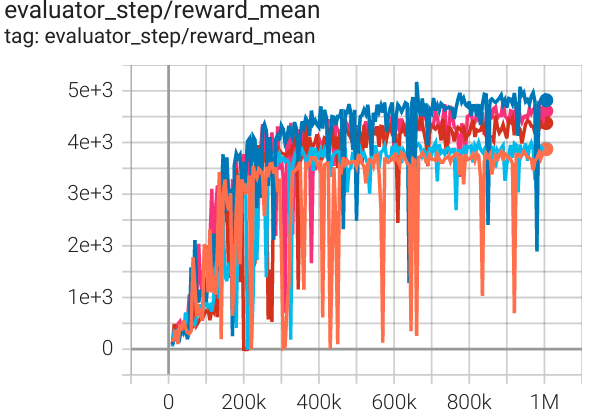
Spinning Up (5300)

SB3(3863)

Tianshou(5007)

Hopper

(Hopper-v2)

3653

config_link_ho

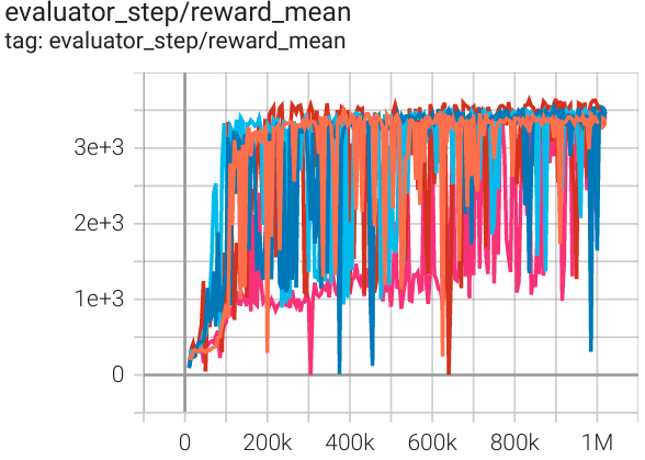
Spinning Up (3500)

SB3(2325)

Tianshou(3542)

Reference¶

Haarnoja, et al. Soft Actor-Critic Algorithms and Applications. [https://arxiv.org/abs/1812.05905 arXiv:1812.05905], 2019.
Haarnoja, et al. Soft Actor-Critic: Off-Policy Maximum Entropy Deep Reinforcement Learning with a Stochastic Actor. [https://arxiv.org/abs/1801.01290 arXiv:1801.01290], 2018.

SAC¶

Overview¶

Quick Facts¶

Key Equations or Key Graphs¶

Pseudocode¶

Extensions¶

Implementation¶

Benchmark¶

Reference¶

Other Public Implementations¶