TD3¶

Overview¶

Twin Delayed DDPG (TD3), proposed in the 2018 paper Addressing Function Approximation Error in Actor-Critic Methods, is an algorithm which considers the interplay between function approximation error in both policy and value updates. TD3 is an actor-critic, model-free algorithm based on the deep deterministic policy gradient (DDPG) that can address overestimation bias, the accumulation of error in temporal difference methods and high sensitivity to hyper-parameters in continuous action spaces. Specifically, TD3 addresses the issue by introducing the following three critical tricks:

Clipped Double-Q Learning: When calculating the targets in the Bellman error loss functions, TD3 learns two Q-functions instead of one, and uses the smaller Q-value.
Delayed Policy Updates: TD3 updates the policy (and target networks) less frequently than the Q-function. In the paper, the author recommends one policy update for two Q-function updates. In our implementation, TD3 only updates the policy and target networks after a ﬁxed number of updates $d$ to the critic. We implement Policy Updates Delay through configuring learn.actor_update_freq.
Target Policy Smoothing: By smoothing out Q along changes in action, TD3 provides noise to the target action, making it more difficult for the policy to exploit Q-function faults.

Quick Facts¶

TD3 is only used for environments with continuous action spaces (e.g., MuJoCo).
TD3 is an off-policy algorithm.
TD3 is a model-free and actor-critic RL algorithm, which optimizes actor network and critic network respectively.

Key Equations or Key Graphs¶

TD3 proposes a clipped Double Q-learning variant which leverages the notion that a value estimate suffering from overestimation bias can be used as an approximate upper-bound to the true value estimate. TD3 shows that target networks, a common approach in deep Q-learning methods, are critical for variance reduction by reducing the accumulation of errors.

Firstly, to address the coupling of value and policy, TD3 proposes delaying policy updates until the value estimate is as small as possible. Therefore, TD3 only updates the policy and target networks after a ﬁxed number of updates $d$ to the critic. We implement Policy Updates Delay through configuring learn.actor_update_freq.

Secondly, the target update of Clipped Double Q-learning algorithm is as follows:

\[y_{1}=r+\gamma \min _{i=1,2} Q_{\theta_{i}^{\prime}}\left(s^{\prime}, \pi_{\phi_{1}}\left(s^{\prime}\right)\right)\]

In implementation, computational costs can be reduced by using a single actor optimized with respect to $Q_{\theta_1}$ . We then use the same target $y_2= y_1for Q_{\theta_2}$.

Finally, a concern with deterministic policies is they can overﬁt to narrow peaks in the value estimate. When updating the critic, a learning target using a deterministic policy is highly susceptible to inaccuracies induced by function approximation error, increasing the variance of the target. TD3 introduces a regularization strategy for deep value learning, target policy smoothing, which mimics the learning update from SARSA. Specifically, TD3 approximates this expectation over actions by adding a small amount of random noise to the target policy and averaging over mini-batches following:

\[\begin{split}\begin{array}{l} y=r+\gamma Q_{\theta^{\prime}}\left(s^{\prime}, \pi_{\phi^{\prime}}\left(s^{\prime}\right)+\epsilon\right) \\ \epsilon \sim \operatorname{clip}(\mathcal{N}(0, \sigma),-c, c) \end{array}\end{split}\]

we implement Target Policy Smoothing through configuring learn.noise, learn.noise_sigma, and learn.noise_range.

Pseudocode¶

\[ \begin{align}\begin{aligned}:nowrap:\\\begin{split}\begin{algorithm}[H] \caption{Twin Delayed DDPG} \label{alg1} \begin{algorithmic}[1] \STATE Input: initial policy parameters $\theta$, Q-function parameters $\phi_1$, $\phi_2$, empty replay buffer $\mathcal{D}$ \STATE Set target parameters equal to main parameters $\theta_{\text{targ}} \leftarrow \theta$, $\phi_{\text{targ},1} \leftarrow \phi_1$, $\phi_{\text{targ},2} \leftarrow \phi_2$ \REPEAT \STATE Observe state $s$ and select action $a = \text{clip}(\mu_{\theta}(s) + \epsilon, a_{Low}, a_{High})$, where $\epsilon \sim \mathcal{N}$ \STATE Execute $a$ in the environment \STATE Observe next state $s'$, reward $r$, and done signal $d$ to indicate whether $s'$ is terminal \STATE Store $(s,a,r,s',d)$ in replay buffer $\mathcal{D}$ \STATE If $s'$ is terminal, reset environment state. \IF{it's time to update} \FOR{$j$ in range(however many updates)} \STATE Randomly sample a batch of transitions, $B = \{ (s,a,r,s',d) \}$ from $\mathcal{D}$ \STATE Compute target actions \begin{equation*} a'(s') = \text{clip}\left(\mu_{\theta_{\text{targ}}}(s') + \text{clip}(\epsilon,-c,c), a_{Low}, a_{High}\right), \;\;\;\;\; \epsilon \sim \mathcal{N}(0, \sigma) \end{equation*} \STATE Compute targets \begin{equation*} y(r,s',d) = r + \gamma (1-d) \min_{i=1,2} Q_{\phi_{\text{targ},i}}(s', a'(s')) \end{equation*} \STATE Update Q-functions by one step of gradient descent using \begin{align*} & \nabla_{\phi_i} \frac{1}{|B|}\sum_{(s,a,r,s',d) \in B} \left( Q_{\phi_i}(s,a) - y(r,s',d) \right)^2 && \text{for } i=1,2 \end{align*} \IF{ $j \mod$ \texttt{policy\_delay} $ = 0$} \STATE Update policy by one step of gradient ascent using \begin{equation*} \nabla_{\theta} \frac{1}{|B|}\sum_{s \in B}Q_{\phi_1}(s, \mu_{\theta}(s)) \end{equation*} \STATE Update target networks with \begin{align*} \phi_{\text{targ},i} &\leftarrow \rho \phi_{\text{targ}, i} + (1-\rho) \phi_i && \text{for } i=1,2\\ \theta_{\text{targ}} &\leftarrow \rho \theta_{\text{targ}} + (1-\rho) \theta \end{align*} \ENDIF \ENDFOR \ENDIF \UNTIL{convergence} \end{algorithmic} \end{algorithm}\end{split}\end{aligned}\end{align} \]

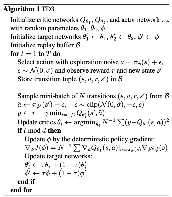
Extensions¶

TD3 is combined with:

Replay Buffers

DDPG/TD3 random_collect_size is set to 25000 by default, while it is 10000 for SAC. We only simply follow SpinningUp default setting and use random policy to collect initialization data. We configure random_collect_size for data collection.

Implementations¶

The default config is defined as follows:

class ding.policy.td3.TD3Policy(cfg: easydict.EasyDict, model: Optional[torch.nn.modules.module.Module] = None, enable_field: Optional[List[str]] = None)[source]¶

Overview:: Policy class of TD3 algorithm. Since DDPG and TD3 share many common things, we can easily derive this TD3 class from DDPG class by changing _actor_update_freq, _twin_critic and noise in model wrapper. Paper link: https://arxiv.org/pdf/1802.09477.pdf

Config:

ID	Symbol	Type	Default Value	Description	Other(Shape)
1	`type`	str	td3	RL policy register name, refer to registry `POLICY_REGISTRY`	this arg is optional, a placeholder
2	`cuda`	bool	False	Whether to use cuda for network
3	`random_` `collect_size`	int	25000	Number of randomly collected training samples in replay buffer when training starts.	Default to 25000 for DDPG/TD3, 10000 for sac.
4	`model.twin_` `critic`	bool	True	Whether to use two critic networks or only one.	Default True for TD3, Clipped Double Q-learning method in TD3 paper.
5	`learn.learning` `_rate_actor`	float	1e-3	Learning rate for actor network(aka. policy).
6	`learn.learning` `_rate_critic`	float	1e-3	Learning rates for critic network (aka. Q-network).
7	`learn.actor_` `update_freq`	int	2	When critic network updates once, how many times will actor network update.	Default 2 for TD3, 1 for DDPG. Delayed Policy Updates method in TD3 paper.
8	`learn.noise`	bool	True	Whether to add noise on target network’s action.	Default True for TD3, False for DDPG. Target Policy Smoo- thing Regularization in TD3 paper.
9	`learn.noise_` `range`	dict	dict(min=-0.5, max=0.5,)	Limit for range of target policy smoothing noise, aka. noise_clip.
10	`learn.-` `ignore_done`	bool	False	Determine whether to ignore done flag.	Use ignore_done only in halfcheetah env.
11	`learn.-` `target_theta`	float	0.005	Used for soft update of the target network.	aka. Interpolation factor in polyak aver -aging for target networks.
12	`collect.-` `noise_sigma`	float	0.1	Used for add noise during co- llection, through controlling the sigma of distribution	Sample noise from dis -tribution, Ornstein- Uhlenbeck process in DDPG paper, Gaussian process in ours.

Model Here we provide examples of ContinuousQAC model as default model for TD3.
class ding.model.ContinuousQAC(obs_shape: Union[int, ding.utils.type_helper.SequenceType], action_shape: Union[int, ding.utils.type_helper.SequenceType, easydict.EasyDict], action_space: str, twin_critic: bool = False, actor_head_hidden_size: int = 64, actor_head_layer_num: int = 1, critic_head_hidden_size: int = 64, critic_head_layer_num: int = 1, activation: Optional[torch.nn.modules.module.Module] = ReLU(), norm_type: Optional[str] = None, encoder_hidden_size_list: Optional[ding.utils.type_helper.SequenceType] = None, share_encoder: Optional[bool] = False)[source]
Overview:
The neural network and computation graph of algorithms related to Q-value Actor-Critic (QAC), such as DDPG/TD3/SAC. This model now supports continuous and hybrid action space. The ContinuousQAC is composed of four parts: actor_encoder, critic_encoder, actor_head and critic_head. Encoders are used to extract the feature from various observation. Heads are used to predict corresponding Q-value or action logit. In high-dimensional observation space like 2D image, we often use a shared encoder for both actor_encoder and critic_encoder. In low-dimensional observation space like 1D vector, we often use different encoders.

Interfaces:
__init__, forward, compute_actor, compute_critic

compute_actor(obs: torch.Tensor) → Dict[str, Union[torch.Tensor, Dict[str, torch.Tensor]]][source]

Overview:
QAC forward computation graph for actor part, input observation tensor to predict action or action logit.

Arguments:

x (torch.Tensor): The input observation tensor data.

Returns:

outputs (Dict[str, Union[torch.Tensor, Dict[str, torch.Tensor]]]): Actor output dict varying from action_space: regression, reparameterization, hybrid.

ReturnsKeys (regression):

action (torch.Tensor): Continuous action with same size as action_shape, usually in DDPG/TD3.

ReturnsKeys (reparameterization):

logit (Dict[str, torch.Tensor]): The predictd reparameterization action logit, usually in SAC. It is a list containing two tensors: mu and sigma. The former is the mean of the gaussian distribution, the latter is the standard deviation of the gaussian distribution.

ReturnsKeys (hybrid):

logit (torch.Tensor): The predicted discrete action type logit, it will be the same dimension as action_type_shape, i.e., all the possible discrete action types.

action_args (torch.Tensor): Continuous action arguments with same size as action_args_shape.

Shapes:

obs (torch.Tensor): $(B, N0)$, B is batch size and N0 corresponds to obs_shape.

action (torch.Tensor): $(B, N1)$, B is batch size and N1 corresponds to action_shape.

logit.mu (torch.Tensor): $(B, N1)$, B is batch size and N1 corresponds to action_shape.

logit.sigma (torch.Tensor): $(B, N1)$, B is batch size.

logit (torch.Tensor): $(B, N2)$, B is batch size and N2 corresponds to action_shape.action_type_shape.

action_args (torch.Tensor): $(B, N3)$, B is batch size and N3 corresponds to action_shape.action_args_shape.

Examples:
>>> # Regression mode >>> model = ContinuousQAC(64, 6, 'regression') >>> obs = torch.randn(4, 64) >>> actor_outputs = model(obs,'compute_actor') >>> assert actor_outputs['action'].shape == torch.Size([4, 6]) >>> # Reparameterization Mode >>> model = ContinuousQAC(64, 6, 'reparameterization') >>> obs = torch.randn(4, 64) >>> actor_outputs = model(obs,'compute_actor') >>> assert actor_outputs['logit'][0].shape == torch.Size([4, 6]) # mu >>> actor_outputs['logit'][1].shape == torch.Size([4, 6]) # sigma

compute_critic(inputs: Dict[str, torch.Tensor]) → Dict[str, torch.Tensor][source]

Overview:
QAC forward computation graph for critic part, input observation and action tensor to predict Q-value.

Arguments:

inputs (Dict[str, torch.Tensor]): The dict of input data, including obs and action tensor, also contains logit and action_args tensor in hybrid action_space.

ArgumentsKeys:

obs: (torch.Tensor): Observation tensor data, now supports a batch of 1-dim vector data.

action (Union[torch.Tensor, Dict]): Continuous action with same size as action_shape.

logit (torch.Tensor): Discrete action logit, only in hybrid action_space.

action_args (torch.Tensor): Continuous action arguments, only in hybrid action_space.

Returns:

outputs (Dict[str, torch.Tensor]): The output dict of QAC’s forward computation graph for critic, including q_value.

ReturnKeys:

q_value (torch.Tensor): Q value tensor with same size as batch size.

Shapes:

obs (torch.Tensor): $(B, N1)$, where B is batch size and N1 is obs_shape.

logit (torch.Tensor): $(B, N2)$, B is batch size and N2 corresponds to action_shape.action_type_shape.

action_args (torch.Tensor): $(B, N3)$, B is batch size and N3 corresponds to action_shape.action_args_shape.

action (torch.Tensor): $(B, N4)$, where B is batch size and N4 is action_shape.

q_value (torch.Tensor): $(B, )$, where B is batch size.

Examples:
>>> inputs = {'obs': torch.randn(4, 8), 'action': torch.randn(4, 1)} >>> model = ContinuousQAC(obs_shape=(8, ),action_shape=1, action_space='regression') >>> assert model(inputs, mode='compute_critic')['q_value'].shape == (4, ) # q value

forward(inputs: Union[torch.Tensor, Dict[str, torch.Tensor]], mode: str) → Dict[str, torch.Tensor][source]

Overview:
QAC forward computation graph, input observation tensor to predict Q-value or action logit. Different mode will forward with different network modules to get different outputs and save computation.

Arguments:

inputs (Union[torch.Tensor, Dict[str, torch.Tensor]]): The input data for forward computation graph, for compute_actor, it is the observation tensor, for compute_critic, it is the dict data including obs and action tensor.

mode (str): The forward mode, all the modes are defined in the beginning of this class.

Returns:

output (Dict[str, torch.Tensor]): The output dict of QAC forward computation graph, whose key-values vary in different forward modes.

Examples (Actor):
>>> # Regression mode >>> model = ContinuousQAC(64, 6, 'regression') >>> obs = torch.randn(4, 64) >>> actor_outputs = model(obs,'compute_actor') >>> assert actor_outputs['action'].shape == torch.Size([4, 6]) >>> # Reparameterization Mode >>> model = ContinuousQAC(64, 6, 'reparameterization') >>> obs = torch.randn(4, 64) >>> actor_outputs = model(obs,'compute_actor') >>> assert actor_outputs['logit'][0].shape == torch.Size([4, 6]) # mu >>> actor_outputs['logit'][1].shape == torch.Size([4, 6]) # sigma

Examples (Critic):
>>> inputs = {'obs': torch.randn(4, 8), 'action': torch.randn(4, 1)} >>> model = ContinuousQAC(obs_shape=(8, ),action_shape=1, action_space='regression') >>> assert model(inputs, mode='compute_critic')['q_value'].shape == (4, ) # q value

Train actor-critic model

Firstly, we initialize actor and critic optimizer in _init_learn, respectively. Setting up two separate optimizers can guarantee that we only update actor network parameters instead of the critic network when we compute actor loss, vice versa.

# actor and critic optimizer
self._optimizer_actor = Adam(
    self._model.actor.parameters(),
    lr=self._cfg.learn.learning_rate_actor,
    weight_decay=self._cfg.learn.weight_decay
)
self._optimizer_critic = Adam(
    self._model.critic.parameters(),
    lr=self._cfg.learn.learning_rate_critic,
    weight_decay=self._cfg.learn.weight_decay
)

In _forward_learn we update actor-critic policy through computing critic loss, updating critic network, computing actor loss, and updating actor network.

critic loss computation

current and target value computation

# current q value
q_value = self._learn_model.forward(data, mode='compute_critic')['q_value']
q_value_dict = {}
if self._twin_critic:
    q_value_dict['q_value'] = q_value[0].mean()
    q_value_dict['q_value_twin'] = q_value[1].mean()
else:
    q_value_dict['q_value'] = q_value.mean()
# target q value. SARSA: first predict next action, then calculate next q value
with torch.no_grad():
    next_action = self._target_model.forward(next_obs, mode='compute_actor')['action']
    next_data = {'obs': next_obs, 'action': next_action}
    target_q_value = self._target_model.forward(next_data, mode='compute_critic')['q_value']

target(Clipped Double-Q Learning) and loss computation

if self._twin_critic:
    # TD3: two critic networks
    target_q_value = torch.min(target_q_value[0], target_q_value[1])  # find min one as target q value
    # network1
    td_data = v_1step_td_data(q_value[0], target_q_value, reward, data['done'], data['weight'])
    critic_loss, td_error_per_sample1 = v_1step_td_error(td_data, self._gamma)
    loss_dict['critic_loss'] = critic_loss
    # network2(twin network)
    td_data_twin = v_1step_td_data(q_value[1], target_q_value, reward, data['done'], data['weight'])
    critic_twin_loss, td_error_per_sample2 = v_1step_td_error(td_data_twin, self._gamma)
    loss_dict['critic_twin_loss'] = critic_twin_loss
    td_error_per_sample = (td_error_per_sample1 + td_error_per_sample2) / 2
else:
    # DDPG: single critic network
    td_data = v_1step_td_data(q_value, target_q_value, reward, data['done'], data['weight'])
    critic_loss, td_error_per_sample = v_1step_td_error(td_data, self._gamma)
    loss_dict['critic_loss'] = critic_loss

critic network update

self._optimizer_critic.zero_grad()
for k in loss_dict:
    if 'critic' in k:
        loss_dict[k].backward()
self._optimizer_critic.step()

actor loss computation and actor network update depending on the level of delaying the policy updates.

if (self._forward_learn_cnt + 1) % self._actor_update_freq == 0:
    actor_data = self._learn_model.forward(data['obs'], mode='compute_actor')
    actor_data['obs'] = data['obs']
    if self._twin_critic:
        actor_loss = -self._learn_model.forward(actor_data, mode='compute_critic')['q_value'][0].mean()
    else:
        actor_loss = -self._learn_model.forward(actor_data, mode='compute_critic')['q_value'].mean()

    loss_dict['actor_loss'] = actor_loss
    # actor update
    self._optimizer_actor.zero_grad()
    actor_loss.backward()
    self._optimizer_actor.step()

Target Network

We implement Target Network trough target model initialization in _init_learn. We configure learn.target_theta to control the interpolation factor in averaging.
# main and target models
self._target_model = copy.deepcopy(self._model)
self._target_model = model_wrap(
    self._target_model,
    wrapper_name='target',
    update_type='momentum',
    update_kwargs={'theta': self._cfg.learn.target_theta}
)

Target Policy Smoothing Regularization

We implement Target Policy Smoothing Regularization trough target model initialization in _init_learn. We configure learn.noise, learn.noise_sigma, and learn.noise_range to control the added noise, which is clipped to keep the target close to the original action.
if self._cfg.learn.noise:
    self._target_model = model_wrap(
        self._target_model,
        wrapper_name='action_noise',
        noise_type='gauss',
        noise_kwargs={
            'mu': 0.0,
            'sigma': self._cfg.learn.noise_sigma
        },
        noise_range=self._cfg.learn.noise_range
    )

Benchmark¶

environment

best mean reward

evaluation results

config link

comparison

HalfCheetah

(HalfCheetah-v3)

11148

config_link_p

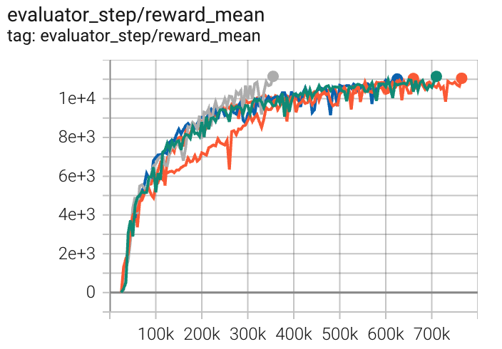
Tianshou(10201) Spinning-up(9750) Sb3(9656)

Hopper

(Hopper-v2)

3720

config_link_q

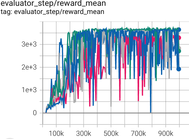
Tianshou(3472) Spinning-up(3982) sb3(3606 for Hopper-v3)

Walker2d

(Walker2d-v2)

4386

config_link_s

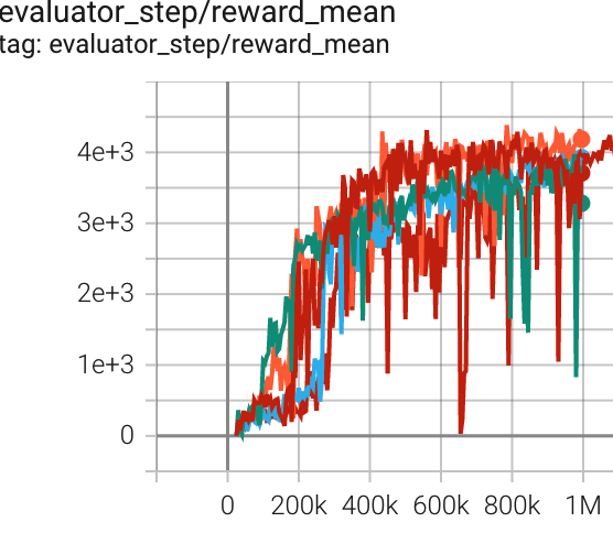
Tianshou(3982) Spinning-up(3472) sb3(4718 for Walker2d-v2)

P.S.：

The above results are obtained by running the same configuration on five different random seeds (0, 1, 2, 3, 4)

References¶

Scott Fujimoto, Herke van Hoof, David Meger: “Addressing Function Approximation Error in Actor-Critic Methods”, 2018; [http://arxiv.org/abs/1802.09477 arXiv:1802.09477].